An algebraic presentation of dialogue categories Paul-Andr Mellis - - PDF document

an algebraic presentation of dialogue categories
SMART_READER_LITE
LIVE PREVIEW

An algebraic presentation of dialogue categories Paul-Andr Mellis - - PDF document

O An algebraic presentation of dialogue categories Paul-Andr Mellis August 22, 2012 Abstract In this paper, we describe an algebraic presentation of the notion of helical dialogue chirality. In particular, the helix structure


slide-1
SLIDE 1

An algebraic presentation

  • f dialogue categories

Paul-André Mellièsú August 22, 2012

Abstract In this paper, we describe an algebraic presentation of the notion of helical dialogue chirality. In particular, the helix structure enables us to decompose the dual of the left negation as the right negation of the dual.

1 Motivations

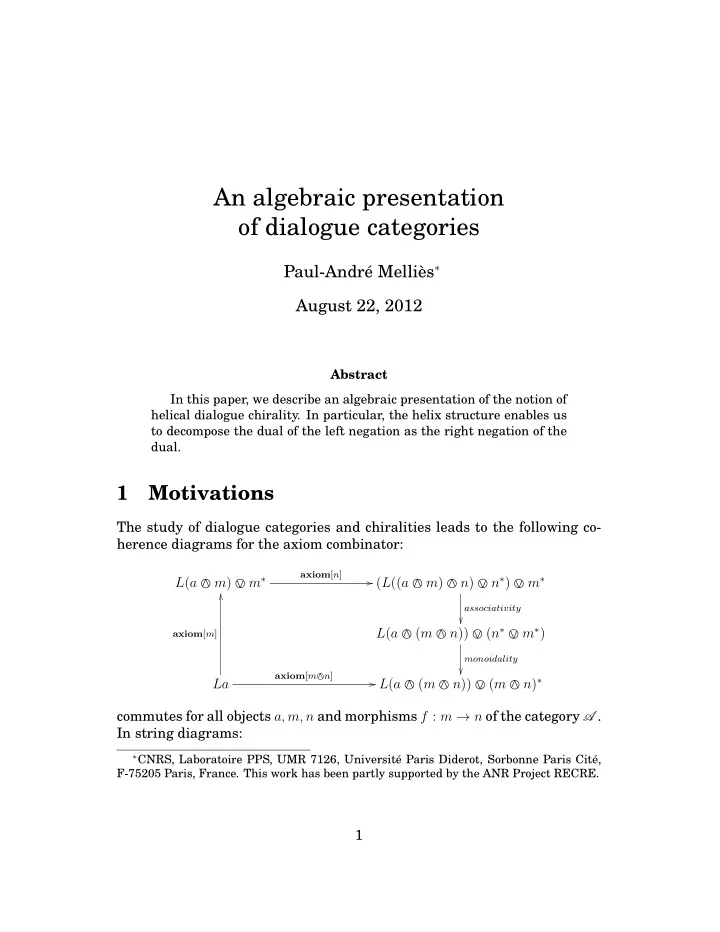
The study of dialogue categories and chiralities leads to the following co- herence diagrams for the axiom combinator: L(a 7 m) 6 mú

axiom[n]

/ (L((a 7 m) 7 n) 6 nú) 6 mú

associativity

L(a 7 (m 7 n)) 6 (nú 6 mú)

monoidality

La

axiom[m]

O

axiom[m7n]

/ L(a 7 (m 7 n)) 6 (m 7 n)ú

commutes for all objects a, m, n and morphisms f : m æ n of the category A . In string diagrams:

∗CNRS, Laboratoire PPS, UMR 7126, Université Paris Diderot, Sorbonne Paris Cité,

F-75205 Paris, France. This work has been partly supported by the ANR Project RECRE.

1

slide-2
SLIDE 2

m L L m n n * *

(a)

=

m L L m n n * * L L

false true

(b)

=

L L

From the logical point of view, the two coherence diagrams (??) and (??) should be understood as η-expansion laws for the axiom link. Typically, the purpose of the η-expansion law (??) is to decompose the link axiom[m 7 n] into the more elementary links axiom[m] and axiom[n]. A natural question is whether there exists a similar η-expansion law which decomposes the axiom link La

right.axiom[Rm]

/

L(a 7 Rm) 6 (Rm)ú associated to the negation of m into the axiom link associated to the ob- ject m of the category B. To that purpose, it appears necessary to start from the left axiom link L(true)

left.axiom[úm] /

(úm)ú 6 L(úm)

equivalence /

m 6 L(úm) associated to the object úm living this time in the category A . Then, the helical structure L(úm)

isomorphism

/

(Rm)ú This defines a morphism La

η

/

L(a 7 RL(true))

map

/

L(a 7 R(m 6 (Rm)ú)) 2

slide-3
SLIDE 3

At this point, we want a map L(a 7 R(m 6 (Rm)ú))

distributivity

/

L(a 7 Rm) 6 (Rm)ú This requires to develop a general theory of these distributivity laws, de- scribing the coherence diagrams.

2 Helical dialogue categories and chiralities

We construct a 2-category of helical dialogue categories, helical functors and helical natural transformations.

2.1 A 2-category of helical dialogue categories

We define a 2-category HelCat with

  • helical dialogue categories as 0-cells,
  • helical functors as 1-cells,
  • dialogue natural transformations as 2-cells.

The 0-dimensional cells. Recall from [6] that a helical dialogue cate- gory C is defined as a dialogue category equipped with a family of bijections wheel x,y : C (x ¢ y, ‹) ≠æ C (y ¢ x, ‹) natural in x and y and required to make the diagram C ((y ¢ z) ¢ x, ‹)

associativity

/ C (y ¢ (z ¢ x), ‹)

wheel y,z¢x

C (x ¢ (y ¢ z), ‹)

wheel x,y¢z

O

associativity

C ((z ¢ x) ¢ y, ‹) C ((x ¢ y) ¢ z, ‹)

wheel x¢y,z

/ C (z ¢ (x ¢ y), ‹)

associativity

O

(1) commute for all objects x, y, z of the category C . 3

slide-4
SLIDE 4

The 1-dimensional cells. A helical functor between two helical dialogue categories is a lax monoidal functor F : C ≠æ D equipped with a morphism ‹F : F(‹) ≠æ ‹ such that the diagram C (x ¢ y, ‹)

F

/

wheel x,y

D(F(x ¢ y), F(‹))

coercion

/ D(F(x) ¢ F(y), ‹)

wheel F (x),F (y)

C (y ¢ x, ‹)

F

/ D(F(y ¢ x), F(‹))

coercion

/ D(F(y) ¢ F(x), ‹)

commutes for all objects x, y of the category C . In this diagram, the two co- ercion maps are deduced by precomposing with the lax monoidal structure

  • f the functor F

mx,y : F(x) ¢ F(y) ≠æ F(x ¢ y) and by postcomposing with the map ‹F. The 2-dimensional cells. A dialogue natural transformation θ : (F, ‹F) ∆ (G, ‹G) is defined as a natural transformation θ : F ∆ G making the diagram F(‹)

θ‹

‹F

' ‹

G(‹)

‹G

7

  • commute. The composition law and identities of the 2-category HelCat are

defined as expected. 4

slide-5
SLIDE 5

2.2 A 2-category of helical dialogue chiralities

We construct a 2-category HelChir with helical dialogue chiralities as 0- cells. The 0-dimensional cells. Definition 1 (Helical chirality) A helical chirality is a dialogue chirality equipped with a family of bijections σa,b : È a | b Í ≠æ È úb | aú Í natural in a, b, and making the diagram below commute: È a1 7 a2 | b Í

χR

a2,a1,b /

σ

È a1 | b 6 aú

2 Í σ

/ È ú(b 6 aú

2) | aú 1 Í

È a2 7 úb | aú

1 Í χR

úb,a2,a1

È úb | (a1 7 a2)ú Í È a2 | aú

1 6 (úb)ú Í

È úb | aú

2 6 aú 1 Í

È úb 7 a1 | aú

2 Í χR

a1,úb,aú 2

  • È ú(aú

1 6 b) | aú 2 Í

È a2 | aú

1 6 b Í σ

  • (2)

The 1-dimensional cells. A 1-dimensional cell in HelChir F : (A1, B1) ≠æ (A2, B2) is defined as a quadruple F = (F•, F¶,  F, F) consisting of a lax monoidal functor F• : A1 ≠æ A2, an oplax monoidal functor F¶ : B1 ≠æ B2, a mo- noidal natural isomorphism A1

F•

/

(≠)ú

✏ Â

F

A2

(≠)ú

✏ 

B op(0,1)

1 F op(0,1)

/ B op(0,1)

2

(3) 5

slide-6
SLIDE 6

together with a natural transformation: A1

F•

/ A2

F

+3

B1

/

R

O

B2

R

O

(4) making the two diagrams È a 7 m | b Í

χm

/

Fa7m,b

È a | b 6 mú Í

Fa,b6mú

È F•(a 7 m) | F¶(b) Í

monoidality of F•

È F•(a) | F¶(b 6 mú) Í

monoidality of F

È F•(a) | F¶(b) 6 F¶(mú) Í

Â

F

È F•(a) 7 F•(m) | F¶(b) Í

χF•(m)

/ È F•(a) | F¶(b) 6 F•(m)ú Í

(5) È a | b Í

Fa,b

/

σa,b

È F•(a) | F¶(b) Í

σF•(a),F¶(b)

È úb | aú Í

Fúb,aú

/ È F•(úb) | F¶(aú) Í Â

F

/ È ú(F¶(b)) | (F•(a))ú Í

(6) commute for all objects a, m in A1 and b in B1. Here, the map Fa,b : È a | b Í ≠æ È F•(a) | F¶(b) Í is defined as the composite È a | b Í

Fa,b

/ È F•(a) | F¶(b) Í

A1(a, Rb)

F•

/

A2(F•(a), F•(Rb))

F

/

A2(F•(a), RF¶(b)) 6

slide-7
SLIDE 7

The 2-dimensional cells. A 2-dimensional cell in HelChir θ : F ∆ G : (A1, B1) ≠æ (A2, B2) is defined as a pair (θ•, θ¶) of monoidal natural transformations θ• : F• ∆ G• and θ¶ : G¶ ∆ F¶ satisfying the two equations below:

θ•

↵◆

A1

F•

(

G•

7

(≠)ú

A2

(≠)ú

✏ Â

G

  • B op(0,1)

1 G op(0,1)

5B op(0,1)

2

= A1

F•

'

(≠)ú

A2

(≠)ú

✏ Â

F

  • θ op(0,1)

↵◆

B op

1 F op(0,1)

)

G op(0,1)

7

B op(0,1)

2

(7) A1

F•

/ A2

F

  • 5

B1

/

R

O

B2

R

O

=

θ•

↵◆

A1

F• G•

/ A2

G

  • 5

B1

/

>

R

O

θ

↵◆

B2

R

O

(8)

2.3 Equivalence

The 2-functor induces a biequivalence between the 2-categories HelCat and HelChir.

3 Helical chiralities revisited

In this section, we study another formulation of helical chiralities.

3.1 Helical dialogue chiralities (bis)

Definition 2 (Helical chirality bis) A helical chirality is a pair of mo- noidal categories (A , 7, true) (B, 6, false) 7

slide-8
SLIDE 8

equipped with a monoidal equivalence A

(≠)ú

"

monoidal equivalence ú(≠)

c

B op(0,1) with two families of bijections χR

m,a,b

: È a 7 m | b Í ≠æ È a | b 6 mú Í χL

m,a,b

: È m 7 a | b Í ≠æ È a | mú 6 b Í natural in a, b and m, where È ≠ | ≠ Í = A ( ≠ , R(≠) ) : A op ◊ B ≠æ Set The families χL and χR are moreover required to make the diagrams below commute: È a 7 (m 7 n) | b Í

χR

m7n

/

associativity

È a | b 6 (m 7 n)ú Í È (a 7 m) 7 n | b Í

χR

n

/ È a 7 m | b 6 nú Í

χR

m

/ È a | (b 6 nú) 6 mú Í

associativity monoidality of negation

O

(9) È (m 7 n) 7 a | b Í

χL

m7n

/

associativity

È a | (m 7 n)ú 6 b Í È m 7 (n 7 a) | b Í

χL

m

/ È n 7 a | mú 6 b Í

χL

n

/ È a | nú 6 (mú 6 b) Í

associativity monoidality of negation

O

(10) together with the additional coherence diagram between χL and χR: È (m 7 a) 7 n | b Í

χR

n

/

associativity

È m 7 a | b 6 nú Í

χL

m

/ È a | mú 6 (b 6 nú) Í

associativity

È m 7 (a 7 n) | b Í

χL

m

/ È a 7 n | mú 6 b Í

χR

n

/ È a | (mú 6 b) 6 nú Í

(11) Proposition 1 The two notions of helical chirality formulated in Defini- tions 1 and 2 are equivalent. 8

slide-9
SLIDE 9

3.2 The 2-category of helical dialogue categories

The 1-dimensional cells. The helical functors may be reformulated in this style. A helical functor is defined as a quadruple F = (F•, F¶,  F, F) consisting of a lax monoidal functor F• : A1 ≠æ A2, an oplax monoidal functor F¶ : B1 ≠æ B2, a monoidal natural isomorphism (3) and a natural isomorphism (4) making the diagram (5) commute for χ = χR together with the corresponding diagram for the left currification χL, given below: È m 7 a | b Í

χL

m

/

Fm7a,b

È a | mú 6 b Í

Fa,mú6b

È F•(m 7 a) | F¶(b) Í

monoidality of F•

È F•(a) | F¶(mú 6 b) Í

monoidality of F

È F•(a) | F¶(mú) 6 F¶(b) Í

Â

F

È F•(m) 7 F•(a) | F¶(b) Í

χL

F•(m)

/ È F•(a) | F•(m)ú 6 F¶(b) Í

(12) The 2-dimensional cells. The 2-dimensional cells are defined as previ-

  • usly for the 2-category HelChir.

3.3 Proof of isomorphism

In order to clarify the comparison between the two definitions of helical dialogue chirality, we decide to call Def-a the original definition 1 and Def- b its alternative but equivalent formulation in Proposition 1. Def-a ∆ Def-b. Every helical dialogue category in the sense of Defini- tion 1 is equipped with a natural bijection σ, In order to obtain a helical dialogue category in the sense of Proposition 1, one defines the natural bi- jection χR as χ and the natural bijection χL as the family of bijections χL

m,a,b

9

slide-10
SLIDE 10

as the composite morphism: È m 7 a | b Í

σ

χL

m,a,b

/ È a | mú 6 b Í

È úb | (m 7 a)ú Í

/ È úb | aú 6 mú Í

χ≠1

m

/ È úb 7 m | aú Í / È ú(mú 6 b) | aú Í

σ≠1

O

Def-b ∆ Def-a. Conversely, given a helical dialogue chirality in the sense

  • f Proposition 1, the natural bijection σ is defined as the unique family of

bijections σa,b making the diagram below commute: È a | b Í

σa,b

/ È úb | aú Í

È a | false 6 (úb)ú Í

(χR

(úb))≠1

/ È a 7 úb | false Í

χL

a

/ È úb | aú 6 false Í O

A series of chase diagrams establish that the relationship is one-to-one.

4 Helical chiralities by transjunctions

Construire une 2-categorie de nouveau, et montrer le lien avec la dualite.

4.1 Definition

It is not difficult to deduce a formulation of helical categories based on tran-

  • sjunctions. This starts with the two coherence diagrams for the right axiom

combinator L(a 7 m) 6 mú

f

  • L(a)

right.axiom[m]

3

right.axiom[n]

+

L(a 7 n) 6 mú L(a 7 n) 6 nú

?

10

slide-11
SLIDE 11

L(a 7 m) 6 mú

right.axiom[n]

/ (L((a 7 m) 7 n) 6 nú) 6 mú

associativity

L(a 7 (m 7 n)) 6 (nú 6 mú)

monoidality

La

right.axiom[m]

O

right.axiom[m7n]

/ L(a 7 (m 7 n)) 6 (m 7 n)ú

followed by the two coherence diagrams for the left axiom combinator mú 6 L(m 7 a)

f

  • L(a)

left.axiom[m]

3

left.axiom[n]

+

mú 6 L(n 7 a) nú 6 L(n 7 a)

?

nú 6 L(n 7 a)

left.axiom[m]

/ nú 6 (mú 6 L(m 7 (n 7 a)))

associativity

(nú 6 mú) 6 L((m 7 n) 7 a)

monoidality

La

left.axiom[n]

O

left.axiom[m7n]

/ (m 7 n)ú 6 L((m 7 n) 7 a)

for every morphism f : m ≠æ n of the category A . Finally, the important additional coherence diagram tells that the tensor products permute: L(a 7 n) 6 nú

left.axiom[m]

/ mú 6 (L(m 7 (a 7 n)) 6 nú)

associativity

L(a)

right.axiom[n]

6

left.axiom[m]

(

mú 6 L(m 7 a)

right.axiom[n]

/ (mú 6 L((m 7 a) 7 n)) 6 nú

11

slide-12
SLIDE 12

4.2 Cut

R(b 6 mú) 7 m

right.cut[m]

R(b 6 nú) 7 m

3

f

+

R(b) R(b 6 nú) 7 n

right.cut[n]

B

(R((b 6 nú) 6 mú) 7 m) 7 n

right.cut[m]

/ R(b 6 nú) 7 n

right.cut[n]

R(b 6 (nú 6 mú)) 7 (m 7 n)

associativity

O

R(b 6 (m 7 n)ú) 7 (m 7 n)

monoidality

O

right.cut[m7n]

/ R(b)

followed by the two coherence diagrams for the left cut combinator m 7 R(mú 6 b)

left.cut[m]

m 7 R(nú 6 b)

3

f

+

R(b) n 7 R(nú 6 b)

left.cut[n]

B

m 7 (n 7 R(nú 6 (mú 6 b)))

left.cut[n]

/ m 7 R(mú 6 b)

left.cut[m]

(m 7 n) 7 R((nú 6 mú) 6 b)

associativity

O

(m 7 n) 7 R((m 7 n)ú 6 b)

monoidality

O

left.cut[m7n]

/ R(b)

12

slide-13
SLIDE 13

for every morphism f : m ≠æ n of the category A . Finally, the important additional coherence diagram tells that the tensor products permute: (m 7 R(mú 6 (a 6 nú))) 7 n

left.cut[m]

/

associativity

nú 6 R(n 7 a)

right.cut[n]

R(b) m 7 (R((mú 6 a) 6 nú) 7 n)

right.cut[n]

/ mú 6 R(m 7 a)

left.cut[m]

O

(13)

4.3 Graphically

The coherence diagram (13) is depicted as

m R R m n n * *

=

m R R m n n * *

4.4 The 2-category

The 1-dimensional cells. A homorphism of helical dialogue chiralities is defined 13

slide-14
SLIDE 14

5 Eta law for negation

5.1 Flexible negation

The following equation holds when the negation is twist-free +

ú(R(false)) 6 L(R(false) 7 true)

/ L(true) 6 L(R(false))

ε

L(true)

axiom≠left

O

axiom≠right

id

/ L(true)

L(true 7 R(false)) 6 ú(R(false))

/ L(R(false)) 6 L(true)

ε

O

6 Discursive pairs

6.1 Definition

A discursive pair is defined as a pair of monoidal categories (A , 7, true) (B, 6, false) equipped with an adjunction A

L

"

R

c

B together with the four bimonads left.κ7 : m 7 R(L(a) 6 b) ≠æ R(L(m 7 a) 6 b) left.κ6 : L(R(n 6 b) 7 a) ≠æ n 6 L(R(b) 7 a) right.κ7 : R(b 6 L(a)) 7 m ≠æ R(b 6 L(a 7 m)) right.κ6 : L(a 7 R(b 6 n)) ≠æ L(a 7 R(b)) 6 n (14) between the 7-tensor product and the B-monad of A on the one hand, and between the 6-tensor product and the A -comonad of B on the other hand. Besides the resulting series of commutative diagrams, we ask that the two diagrams below commute 14

slide-15
SLIDE 15

κ left. κ left.

a R R L m n L a R L m n L R a R L m L n R b b b R L m L n R a b a R L m L n R b

κ left. κ left. κ left.

a R R L n m L a R L n m L R a R L n L m R a R L n L m R R L n L m R a b b b b b

κ right. κ right. κ right. κ right. κ right.

for all objects a, m, n of the category A and all object b of the category B. Plus a series of other diagrams required in the proof of the following lemma.

R R a b L m

κ right.

R R a b L m

κ left.

R R a b L m

κ left. κ right.

R R a b L m

15

slide-16
SLIDE 16

Note that these coherence diagrams are not justified by any of the previous discussions.

7 Dualities

A duality in a discursive pair (A , B) is defined as a monoidal equivalence A

(≠)ú

"

monoidal equivalence ú(≠)

c

B op(0,1) together with four families of morphisms right.AX[m] : true ≠æ R(L(m) 6 mú) right.CUT[m] : L(R(mú) 7 m) ≠æ false left.AX[m] : true ≠æ R(mú 6 L(m)) left.CUT[m] : L(m 7 R(mú)) ≠æ false each of them parametrized by the objects m of the category A . These mor- phisms are required to make the three coherence diagrams below commute. The right coherence diagrams. The first coherence diagram adapts the usual triangular axiom of adjunctions:

L m * L m R m L m * L m R m L m L m

id right.AX m right.CUT m κ left.

The second coherence diagram means that the family of combinators AX[≠] is dinatural: 16

slide-17
SLIDE 17

* R m L m * R n L n * m L n * f true R f

right.AX n right.AX m

The third coherence diagram expresses a monoidality of the family AX[≠]:

true * R m L m * R m L m * R n L n

right.AX m

n R L m n * m * n * R m L m * R n L n

ε right.AX n right.AX m κ left.

true * R L

η right.AX

true true R L true false R L true

monoidality

  • f

negation unit law

true

The four coherence diagrams hold for all objects m, n and all morphisms f : m æ n of the category A . The left coherence diagrams. We need to give the same coherence dia- grams on the left side. 17

slide-18
SLIDE 18

L m * L m R m L m * L m R m L m L m

id left.AX m left.CUT m κ right.

* R m L m * R n L n * m L n * f true R f

left.AX n left.AX m

true * R n L n * R n L n * R m L m

left.AX m

n R L m n * m * n * R n L m * R m L n

ε κ right. left.AX n left.AX m

true * R L

η left.AX

true true R L true false R L true

monoidality

  • f

negation unit law

true

18

slide-19
SLIDE 19

The mixed coherence diagrams. We also ask this one, which ensures that the two left and right axioms commute:

right.AX

* R m L m n * R n L n true * R n L n * R m L m m

left.AX

m

left.AX right.AX n

* R n L n * R m L m * R n L n * R m L m * R n L n * R m L m * R n L n * R m L m

κ right. κ left. κ right. κ left.

(15) Remark. These coherence diagrams should be dualized and repeated for the combinator CUT. There is apparently no way to recover them from the coherence diagrams for the combinator AX.

8 Main theorem

8.1 Preliminary result on helicality

One main benefit of introducing the coherence diagram (??) is that we can establish the following property, which states that the dialogue category is helical. Proposition 2 Suppose given a discursive pair with a duality. In that case, the following diagram

a L

right.AX n κ left.

a * n L n

ε κ right. left.AX m κ right. ε

a * m L m

right.AX n κ left. left.AX m ε ε

a * n n * L m m

19

slide-20
SLIDE 20

commutes. The proof that the left and the right axioms commute is based on the com- mutative diagram below:

R L a L

right.AX n

a L

κ left.

* R n L n a L * R n L n a * n L n

ε

a * n L n

η η

R L a * n L n R

ε η

a L * R n L n L R L

κ left. η

a L R L true

right.AX n

a L R L * R n L n

κ right. κ left.

a L R L * R n L n

ε

a L * R n L n

right.AX n

a L R * n L n

η η id κ right. κ right.

Note that we only need a special case of Diagram (??) with η in front of AX[n]. This commutative diagram enables to establish in turn that the diagram below commutes:

a L

right.AX n κ left.

a * n L n

ε κ right. left.AX m κ right. ε

a * m L m

right.AX n κ left. left.AX m ε ε

a * n n * L m m

η η

a * n n * L m m L R L R a * n n * L m m

η η right.AX n left.AX m

a L * m L m R a L * m L m R * n L n R

κ right. κ left.

20

slide-21
SLIDE 21

In order to conclude, there simply remains to establish that the two mor- phisms η appearing in the previous diagram are monos. This immediately follows from the fact that

a n L m L R L R a n L m

κ right. κ left. ε ε η η

a n L m L R L R a n m L

is equal to the identity., this esta that each η morphism involved in the previous diagram are monos. We conclude that the expected diagram

a L

right.AX n κ left.

a * n L n

ε κ right. left.AX m κ right. ε

a * m L m

right.AX n κ left. left.AX m ε ε

a * n n * L m m

commutes. Corollary 3 Suppose given a helical discursive pair with a helical duality. In that case, the induced dialogue chirality is helical. There remains to show that...

8.2 From chiralities to discursive pairs and back

Given a helical chirality, one constructs a helical discursive pair equipped with a duality. Proposition 4 The helical chirality deduced from the helical discursive pair and its duality coincide with the original helical chirality. This is easy. This essentially reduces to establishing that the morphism right.axiom[m] : L(a) ≠æ L(a 7 m) 6 mú in the original helical chirality (A , B) coincides with the morphism L(a)

right.AX[m] / left.κ7

/

ε

/ L(a 7 m) 6 mú

21

slide-22
SLIDE 22

recovered from the associated discursive pair. This is established by the simple diagram chase below

a L η

left.axiom a left.cut a

true R L a L R L a L a * a R L L a * R m L m a L

right.AX m left.axiom a left.cut a

* R m L m a L a * a * R m L m a L ε * m L m a a L η a L ε

id id κ left. right.axiom m right.axiom m right.axiom m

(16) One then needs to check that the morphisms left.axiom[m], right.cut[m] and left.cut[m] coincide with their reconstruction in the discursive pair. Each of the three facts is established by one of the three possible symmetric variants of the diagram (16).

8.3 From discursive pairs to chiralities and back

Suppose given a helical discursive pair equipped with a duality. We have seen how to construct a helical chirality from it. The question we would like to address here is whether the associated discursive pair coincides with the

  • riginal one. The first step is to check that the morphism

right.AX[m] : true ≠æ R(L(m) 6 mú)

  • f the original duality coincides with the morphism

η true R L ε true

right.AX m κ left.

true R L * R m L m R L * R m L m * R m L m

22

slide-23
SLIDE 23

which corresponds to the morphism reconstructed from the chirality. This is essentially immediate. One needs to do the same for the three other com- ponents left.AX[m], right.CUT[m] and left.CUT[m] of the original duality. This is done in just the same way, by applying the appropriate symmetry to the case just treated. Now, the main difficulty lies in the second part of the proof, which con- sists in establishing that the distributivity law right.κ7 : R(b 6 L(a)) 7 m ≠æ R(b 6 L(a 7 m))

  • f the original discursive pair coincides with the morphism reconstructed

from the associated chirality. This amounts to establishing that the dia- gram below

η

κ left.

R L a m b

right.AX m

R L a m b * R m L m R L a m b * R m L m ε R a m b * m L m R a m b * m L m L R

κ left.

R a m b * m L m L R

right.CUT

m a b L m R

κ right.

  • commutes. This is true, but not so easy to establish, although it boils down

to producing the appropriate diagram chase. We start by establishing that

a L m * R m L m a L m a L m L a m * R m L m L a m * R m L m

right.CUT

m

right.AX m κ left. κ left. id

23

slide-24
SLIDE 24

commutes as follows:

a m R L

id right.AX m

* R m L m a L m R

κ left.

* R m L m a L m R L m a R L a m * R m L m

κ left.

R

κ left. right.CUT

m

right.CUT

m a m R L a m η η

κ l e f t . r i g h t . A X

m

κ l e f t .

* R m L m a L m R

κ left.

* R m L m a L m R

κ l e f t .

η a m R L

We then observe that the diagram below

right.CUT

m false ε false R L L m * R m R L * R m L m

right.CUT

m ε L m * R m R L false

κ right.

L m * R m R L

κ right.

commutes, as an instance of Then, we get the final diagram chase: 24

slide-25
SLIDE 25

8.4 Main result (step 4)

Proposition 5 There is a one-to-one relationship between the two following notions:

  • a helical dialogue chirality,
  • a helical discursive pair equipped with a duality.

References

[1] Richard Blute, Robin Cockett, Robert Seely, and Todd Trimble. Natural de- duction and coherence for weakly distributive categories. Journal of Pure and Applied Algebra, 113:229?296, 1996. [2] Robin Cockett, Robert Seely. Polarized category theory, modules, and game

  • semantics. Theory and Applications of Categories 18 (2) (2007) 4–101.

[3] Max Kelly, Ross Street. Review of the elements of 2-categories, in Kelly (ed.), Category Seminar, LNM 420. [4] Paul-André Melliès. Categorical semantics of linear logic. Published in Interac- tive models of computation and program behaviour. Pierre-Louis Curien, Hugo Herbelin, Jean-Louis Krivine, Paul-André Melliès. Panoramas et Synthèses 27, Société Mathématique de France, 2009. [5] Paul-André Melliès. Dialogue categories and chiralities. Submitted. Manuscript available on the author’s webpage. [6] Paul-André Mellies. Braided notions of dialogue categories. Submitted. Manuscript available on the author’s webpage.

25

slide-26
SLIDE 26

Diagram

κ left.

R L a m b

right.AX m

R L a m b * R m L m R L a m b * R m L m a b L m R

κ right. κ right. right.AX m

* R m L m a b L m R

κ right.

R L a m b * R m L m

κ left.

η R L a m b * R m L m L R ε R a m b * m L m L R R a m b * m L m L R

right.CUT

m a b L m R

κ right.

R L a m b * R m L m L R η R L a m b * R m L m L R

κ left. κ left. κ right.

R L a m b * R m L m L R R L a m b * R m L m L R

κ left.

R L a m b * R m L m L R ε

κ left.

R L a m b * R m L m L R

κ left. κ right. κ right.

R L a m b * R m L m L R

right.CUT

m R a b L m L R a b L m R L R * R m L m a b L m R L R R a b L m L R * R m L m a b L m R L R

κ left.

η η

right.AX m κ left. κ left. right.AX m id

ε

κ left. κ left. κ left. κ left.

R a m * m L m L b R ε ε ε L a m b * R m L m R

right.CUT

m

right.CUT

m

κ left.

a b L m R R L false L m * R m R L false

κ right.

a b L m R ε

Diagram

ε ε

id

Figure 1: Commutative diagram 26

slide-27
SLIDE 27

. 27

slide-28
SLIDE 28

9 Appendix

9.1 Main proposition

Proposition 6 Every helical chirality (A , B) comes equipped with the nat- ural transformations right.κ7 : R(b 6 L(a)) 7 m ≠æ R(b 6 L(a 7 m)) right.κ6 : L(a 7 R(b 6 n)) ≠æ L(a 7 R(b)) 6 n left.κ7 : m 7 R(L(a) 6 b) ≠æ R(L(m 7 a) 6 b) left.κ6 : L(R(n 6 b) 7 a) ≠æ n 6 L(R(b) 7 a) natural in a, m and b, defined as R(b 6 L(a)) 7 m

right.κ7

/

right.axiom[m]

R(b 6 L(a 7 m)) R(b 6 (L(a 7 m) 6 úm)) 7 m

associativity

/ R((b 6 L(a 7 m)) 6 úm) 7 m

right.cut[m]

O

L(a 7 R(b 6 n))

right.κ6

/

right.axiom[ún]

L(a 7 R(b)) 6 L((a 7 R(b 6 n)) 7 ún) 6 (ún)ú

equivalence / L((a 7 R(b 6 n)) 7 ún) 6 n associativity / L(a 7 (R(b 6 n) 7 right cu

O

and similarly for left.κ7 and left.κ6. They define together a helical dialogue chirality.

10 Dualities

10.1 Definition

A duality on a linearly distributive pair (A , B) is defined as a monoidal equivalence A

(≠)ú

"

monoidal equivalence ú(≠)

c

B op(0,1) 28

slide-29
SLIDE 29

together with four families of morphisms right.AX[m] : true ≠æ R(L(m) 6 mú) right.CUT[m] : L(R(mú) 7 m) ≠æ false left.AX[m] : true ≠æ R(mú 6 L(m)) left.CUT[m] : L(m 7 R(mú)) ≠æ false each of them parametrized by the objects m of the category A . These mor- phisms are moreover required to make the coherence diagrams below com- mute.

L m * L m R m L m * L m R m L m L m

κ right.AX right.CUT id left.

true * R m L m

right.AX κ η right.AX

* R m L m * R n L n * R m L m * R n L n R L m n * m * n

right.AX κ

R L m n * m * n R L true * R L

η right.AX

true true R L true false R L true

monoidality

  • f

negation unit law

29

slide-30
SLIDE 30

right.AX

* R m L m

right.AX

* R n L n * m L n * f f true R

for all objects m, n and all morphisms f : m æ n of the category A .

10.2 Main proposition

Proposition 7 Every helical dialogue chirality comes equipped with a du- ality defined as follows: right.AX[m] : true

η /

RL(true)

right.axiom[m] /

R(L(m) 6 mú) right.CUT[m] : L(R(mú) 7 m)

right.cut[m]

/

L(R(false)

ε /

false left.AX[m] : true

η /

RL(true)

left.axiom[m] /

R(mú 6 Lm) left.CUT[m] : L(m 7 R(mú))

left.cut[m]/

L(R(false)

ε /

false Remark. For simplicity, we do not mention the monoidal coercions when they are obvious. Typically, in full rigor, the right axiom map is defined as follows: true

η

/ RL(true)

right.axiom[m] / R(L(true 7 m) 6 mú) unit / R(L(m) 6 mú)

11 A reconstruction of helical chiralities

We show that a distributive pair equipped with a duality is the same thing as a dialogue chirality. Theorem 1 A helical chirality is the same thing as a linearly distributive pair equipped with a duality. 30

slide-31
SLIDE 31

Proof of one of the triangular law

a m R L a m R L a m * R L a m R m L m * R L a m R m L m * R L a m R m L m R a L m * R L a m R m L m * R L a m R m L m

η η κ κ κ κ κ κ

R a L m

AX AX CUT CUT id κ

Proof of monoidality

a * a R m L m

AX κ

* R m L m a * R m L m * a R n L n * R m L m * a R n L n

ε

* R m m * a n L n

AX κ

* R m L m * R n L n a * R m L m * R n L n a a R L m n * m * n

AX κ κ AX

* R m L m * R n L n a

κ κ κ ε

Proof of naturality 31

slide-32
SLIDE 32

a

AX

* a R m L m

AX

* a R n L n

κ κ

* a R m L m * a R n L n * a R m L n * a R m L n

κ

* f * f f f

The proof of commutation is more involved. First of all, we observe that the diagram below commutes.

true * R m L m

right.AX κ η right.AX

* R m L m * R n L n * R m L m * R n L n R L m n * m * n

right.AX κ

R L m n * m * n R L

Then. 32

slide-33
SLIDE 33

a

AX

* a R m L m

AX

* a R n L n

κ

* a R n L n

κ

* a R m L m

AX AX

* a R m L m * R n L n * a R n L n * R m L m

κ κ

* a R m L m * R n L n * a R n L n * R m L m * a R m m * n L n

ε ε κ

* a R m L m * R n L n

AX κ AX

11.1 Eta-expansion of negation

Check that the diagram below commutes. L(a 7 R(m 6 L(úm)))

κ

*

L(a 7 RL(true))

left.axiom[úm]

5

L(a 7 R(m)) 6 L(úm)

La

η

O

right.axiom[Rm]

/ L(a 7 Rm) 6 (Rm)ú

L(R(L(úm) 6 m) 7 a)

κ

*

L(RL(true) 7 a)

right.axiom[úm]

5

L(úm) 6 L(R(m) 7 a)

La

η

O

left.axiom[Rm]

/ (Rm)ú 6 L(R(m) 7 a)

33

slide-34
SLIDE 34

12 The balanced and symmetric cases

In that case, all the left structures are deduced using the braiding. This has to be done very carefully. 34