Algorithm of Abnormal Event Diagnosis with the Identification of - - PDF document

Transactions of the Korean Nuclear Society Virtual Spring Meeting July 9-10, 2020

Algorithm of Abnormal Event Diagnosis with the Identification of Unknown Events and Output Confirmation Hyojin Kim and Jonghyun Kim*

*Department of Nuclear Engineering, Chosun University, 309 pilmun-daero, Dong-gu, Gwangju, 501-709, Republic

• f Korea

*Corresponding author: jonghyun.kim@chosun.ac.kr

• 1. Introduction

Diagnosis in abnormal situations is known to be one

• f the difficult tasks in nuclear power plants (NPPs). To

begin with, there is too much information to consider when operators make decisions. NPPs have not only approximately 4,000 alarms and monitoring devices in the main control room (MCR) but also more than one hundred operating procedures for abnormal situations [1]. These information overloads could confuse operators as well as increase the likelihood of error caused by an increase in the mental workload of operators. In addition, some abnormal situations require a very quick diagnosis and response to prevent the reactor from being tripped. To deal with these issues, several researchers have developed operator support systems and algorithms to reduce burdens for operators using computer-based and artificial intelligence (AI) techniques, such as support vector machines (SVM), expert systems, and artificial neural networks (ANNs) [2-4]. Among them, ANNs are regarded as one of the most relevant approaches to handle pattern recognition as well as huge nonlinear data. Thus, several studies have proposed diagnostic algorithms using ANNs [2]. Even though several diagnostic algorithms using ANNs have performed well in trained cases, there are some potential improvements. One of them is that unknown events are not identified as “unknown” because an ANN algorithm that is trained with the supervised learning tries to generate one of trained cases even if it is not trained. Therefore, there is a potential that the algorithm produces wrong results when untrained events

• ccur. This may mislead operators when the algorithm is

involved in an operator support system. Another is that an algorithm cannot confirm whether its outputs are reliable or not. The previously developed algorithm provides multiple diagnosis results with a probability or confidence [2]. This may impose another burden on operators because they have to verify which diagnosis result is consistent with the current situation. In this light, this study aims to propose a diagnostic algorithm for abnormal situations in NPPs that can identify unknown events and confirm results itself. The diagnostic algorithm uses long short-term memory (LSTM) and variational autoencoder (VAE). LSTM is applied for diagnosing abnormal situations as a primary

• network. VAE based assistance networks are applied for

identifying an unknown event and confirming diagnosis

• results. The diagnostic algorithm for abnormal situations

is implemented, trained, and tested for the demonstration using the compact nuclear simulator (CNS).

• 2. Methodology

2.1. Long Short Term Memory LSTM is a special kind of recurrent neural networks (RNNs), capable of learning long-term dependency

• problem. A most distinctive feature of LSTM, compared

to conventional RNNs, is the gate structure. The gate structure consists of an input gate, forget gate, and an

• utput gate. The output from the input is regulated by

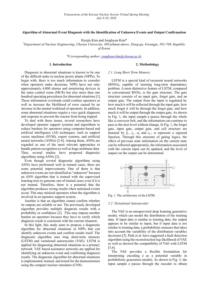
how much it will be reflected through the input gate, how much forget it will be through the forget gate, and how much it will be output through the output gate. As shown in Fig. 1, the input sample 𝑦 passes through the whole like a conveyor belt, and the information can continue to pass to the next level without change. In Fig. 1, the forget gate, input gate, output gate, and cell structure are denoted by 𝑔

𝑢 , 𝑗𝑢 , 𝑝𝑢 and 𝑑𝑢 σ represent a sigmoid

• function. Through this structure of gating logics, the

effect of previous state information on the current state can be reflected appropriately, the information associated with the current input can be updated, and the level of impact on the output can be determined.

• Fig. 1. The architecture of the LSTM.

2.2. Variational Autoencoder The VAE is an unsupervised deep learning generative model, which can model the distribution of the training

• data. If input data is similar to training data, the output

appears to be similar to input, but if input data is not similar to training data, a probabilistic measure that takes into account the variability of the distribution variables decreases [5]. Park et al. have suggested a fault detection algorithm using the reconstruction log-likelihood of VAE as well as showed the compatibility of VAE with LSTM [5,6]. The VAE provides a flexible formulation for interpreting encoding 𝑨 as a potential variable in probabilistic generation models. As shown in Fig. 3, the input sample 𝑦 passes through the encoder to obtain

Transactions of the Korean Nuclear Society Virtual Spring Meeting July 9-10, 2020

parameters of the latent space distribution. The latent variable 𝑨 is obtained from sampling in the current distribution, then 𝑨 is used to generate a reconstructed sample through the decoder [6]. It is comprised of a probabilistic encoder (𝑟𝜚(𝑨|𝑦)) and a decoder (𝑞𝜄(𝑦|𝑨)). Since the posterior distribution (𝑞𝜄(𝑨|𝑦)) is intractable, the VAE approximates 𝑞𝜄(𝑨|𝑦) using the encoder 𝑟𝜚(𝑨|𝑦) , which is assumed to be Gaussian and is parameterized by ∅ and the encoder learns to predict latent variables 𝑨 . As a result, it becomes possible to draw samples from this distribution. To decode a sample 𝑨 drawn from 𝑟𝜚(𝑨|𝑦) , to the input 𝑦, the reconstruction loss (as shown in Eq. (1)) also needs to be minimized. The first term of Eq. (1) is the KL divergence between the approximate posterior and the prior latent variable 𝑨. The second term of Eq. (1) can be understood in terms of the reconstruction of 𝑦 through the posterior distribution 𝑟𝜚(𝑨|𝑦) and the likelihood 𝑞𝜄(𝑦|𝑨) [5]. 𝑀(𝜄, 𝜚; 𝑦(𝑗)) = −𝐸𝐿𝑀(𝑟𝜚(𝑨|𝑦(𝑗))||𝑞𝜄(𝑨)) + 𝔽𝑟𝜚(𝑨|𝑦(𝑗))[𝑚𝑝𝑕𝑞𝜄(𝑦|𝑨)] (1)

• Fig. 2. The architecture of the VAE.
• 3. Development of an Abnormal Diagnosis

Algorithm This chapter suggests a diagnostic algorithm for abnormal situations using LSTM and VAE. Fig. 3 shows the process of the algorithm. It comprises 4 steps Step 1) input preprocessing, Step 2) unknown event identification, Step 3) event diagnosis, Step 4) confirmation of diagnosis results. The details of each step are as below.

• Fig. 3. Overview of a diagnostic algorithm for the abnormal

situation.

3.1 Input preprocessing The first step of the algorithm is to process plant parameters to be suitable for the input of networks. The inputs for the LSTM and VAE networks are selected based on procedures and their importance that can affect the plant states and system availability. These inputs should have a range of values from 0 to 1. However, plant parameters have different ranges of values. Generally, variables with higher values will have more impact on the result of networks. However, this does not necessarily mean that this is more important as a

• predictor. This problem makes local minima. The min-

max normalization can help prevent local minima and also increases the learning speed. Thus, the input to the networks is calculated by Eq. (2). 𝑦𝑢 is the current value

• f plant parameters while 𝑦𝑛𝑏𝑦 and 𝑦𝑛𝑗𝑜 are the

maximum and minimum values of collected data,

• respectively. Through this equation, the input has a range
• f 0 to 1.

𝑦𝑜𝑝𝑠𝑛 = (𝑦𝑢 − 𝑦𝑛𝑗𝑜)/(𝑦𝑛𝑏𝑦 − 𝑦𝑛𝑗𝑜) (2) 3.2 Unknown event identification This step is to identify the unknown event using combining VAE and LSTM. Fig. 4 shows an overview process of unknown event identification. This study defines the anomaly score using negative log-likelihood. If the anomaly score is below the threshold, the event is identified as a known event for which the diagnosis network in the next step has been trained. If the anomaly score is above the threshold, the event is unknown. In this study, the threshold is determined using a three-sigma limit.

• Fig. 4. The process of unknown event identification.

3.3 Event diagnosis This step produces diagnostic results for the plant situation using an LSTM network. Fig. 5 shows the process of diagnosing events. This LSTM receives normalized plant parameters and produces identified events for the abnormal situation with their probabilities. Then, the output is post-processed by using the softmax

• function. The softmax function is an activation function

commonly used in the output layer of the deep learning

• model. Then, This step chooses the event of the highest

probability and provides it for the next step, i.e., the confirmation of diagnosis results.

• Fig. 5. The process of event diagnosis.

Transactions of the Korean Nuclear Society Virtual Spring Meeting July 9-10, 2020

3.4 Confirmation of diagnosis results This step is to confirm whether the current abnormal situation is identical to the event selected in the previous

• step. Fig. 6 shows the process of confirmation of

diagnosis results. The confirmation algorithm has a library of VAE networks that already have been trained. This step selects the VAE network from the library for the event identified in the previous step. Then, it checks whether the current situation is identical to the event expected by the selected VAE. If the anomaly score is below the threshold, the algorithm declares that the diagnosis results in the previous step are correct and

• confirmed. If the anomaly score goes beyond the

threshold, it returns to the previous step. This step also determines each threshold using a three-sigma limit similar way to Step 2).

• Fig. 6. The process of confirmation of diagnosis results.
• 4. Experiment

This study implemented the suggested algorithm by using an NPP simulator. 4.1 Data collection In order to build, train, and validate the suggested algorithm, a compact nuclear simulator (CNS) was used as a real-time testbed. The CNS references a Westinghouse 900MWe, three loops, pressurized water

• reactor. Total 20 abnormal situations and 558 cases are

simulated to collect data. Table 1 shows the abnormal scenarios and the numbers of simulations for each even. The scenarios include representative abnormal situations in actual NPPs such as instrument failures (1 to 6), component failures (7 to 16), and leakages (17 to 20). Based on the abnormal operating procedures of reference plant, 139 parameters were selected for the inputs, including plant variables (e.g., temperature or pressure) and component states (e.g., pump or valve status). The 139 parameters are collected every second in the simulated cases. Among 20 scenarios collected, 409 cases of 15 scenarios, except five scenarios for validating untrained events, are used for training. Then, total 149 cases are used for the validation of algorithm, including five untrained events, i.e., 3, 13, 14, 15, and 20. In addition, to be similar to the real NPPs data, Gaussian noise with 5% is added to the collected data

Table I: Scenarios

No. Scenarios Cases 1 Fail of Pressurizer pressure channel (High) 18 2 Fail of Pressurizer pressure channel (Low) 27 3 Fail of Pressurizer water level channel (High) 6 4 Failure of pressurizer water level channel (Low) 15 5 Failure of steam generator water level channel (Low) 40 6 Failure of steam generator water level channel (High) 42 7 Control rod drop 48 8 Continuous insertion of control rod 8 9 Continuous withdrawal of control rod 8 10 Opening of pressurizer PORV 52 11 Failure of pressurizer safety valve 51 12 Open of pressurizer spray valve 50 13 Stopping of charging pump 1 14 Stopping of 2 main feedwater pumps 3 15 Main steam line isolation 3 16 Rupture of front part regenerative heat exchanger 50 17 Leakage from chemical volume and control system (CVCS) to Component Coolant Water (CCW) 50 18 Leakage at the outlet of charging control flow valve 30 19 Leakage into the CCW system from Reactor Coolant System (RCS) 30 20 Leakage from steam generator tube 36 Total 568

4.2 Training and optimization As mentioned above, total 409 scenarios (i.e., 191,566 datasets for 139 parameters) are trained. In order to

• ptimize the LSTM network in Step 3). Diagnosis, this

study used the manual search method, adjusting the hyperparameters one by one (it is known that there is no golden rule for hyperparameter determinization to

• ptimize the network). Table Ⅱ shows the accuracy

comparison results for the different structures of

• networks. The accuracy is defined by Eq. (3). The LSTM

network with 10 input sequence lengths, 3 layers, and 32 batch sizes is selected.

Table Ⅱ: Accuracy comparison results between networks

No. Sequence Batch sizes Layers Accuracy 1 5 32 2 0.9668 2 5 32 3 0.9638 3 5 64 2 0.9634 4 5 64 3 0.9650 5 10 32 2 0.9768 6 10 32 3 0.9746 7 10 64 2 0.9764 8 10 64 3 0.9741

𝐵𝑑𝑑𝑣𝑠𝑏𝑑𝑧 = 𝑑𝑝𝑠𝑠𝑓𝑑𝑢𝑚𝑧 𝑞𝑠𝑓𝑒𝑗𝑑𝑢𝑓𝑒 𝑒𝑏𝑢𝑏 𝑢𝑝𝑢𝑏𝑚 𝑢𝑓𝑡𝑢𝑗𝑜𝑕 𝑒𝑏𝑢𝑏 (3)

The algorithm has 17 VAE networks, i.e., one for Step 2 Unknown Event Identification and 16 for Step 4

• Confirmation. The VAE network was trained until the

cosine similarity was more than 0.99. Cosine similarity is a measure of similarity between two non-zero vectors

• f an inner product space that measures the cosine of the

angle between them. The cosine of 0° is 1, and it is less

Transactions of the Korean Nuclear Society Virtual Spring Meeting July 9-10, 2020

than 1 for any angle. Cosine similarity is defined by Eq. (4). 𝑌𝑗 is the value of plant parameters at time 𝑗 and 𝑌

̂𝑗 is

the value of restored 𝑌𝑗 at time 𝑗 by VAE.

𝐷𝑝𝑡𝑗𝑜𝑓 𝑡𝑗𝑛𝑗𝑚𝑏𝑠𝑗𝑢𝑧 = ∑ 𝑌𝑗 ∗ 𝑌 ̂𝑗

𝑜 𝑗=1

√∑ (𝑌𝑗)2 ∗

𝑜 𝑗=1

√∑ (𝑌 ̂𝑗)2

𝑜 𝑗=1

(4)

4.3 Validation A validation has been carried out for 149 scenarios (i.e., 58,109 datasets). Among them, 100 cases and 47,872 datasets are used for the trained events while 49 cases and 10,237 datasets are for untrained events. The validation showed that the implemented algorithm produced correct results for all the test cases. Fig. 7 illustrates how the algorithm works for diagnosing a trained event which is Ab 08, continuous insertion of control rod. Step 1) normalizes plant parameters, and then Step 2) identifies the current situation as a trained

• event. Step 3) diagnoses the event as Ab 08 and Step 4)

confirms that this diagnosis result is correct. Finally, “Ab

• 08. Continous insertion of control rod” is presented as

the diagnosis result for the current situation.

• Fig. 8 show an illustration for diagnosing an untrained

event, which is Ab 20, leakage from steam generator tube. In this case, Step 2) identifies the event as an untrained because the construction error goes beyond the threshold. Thus, the message “Unknown Even” is provided.

• Fig. 7 An illustration for diagnosing an trained event
• Fig. 8 An illustration for diagnosing an trained event
• 5. Conclusion

This study has proposed an algorithm that uses LSTM and VAE to diagnose abnormal situations in NPPs. The suggested algorithm has a capability of judging unknown situations, diagnosing the situation and confirming the

• result. In addition, for more realistic algorithm, noise-

added signals are also considered. The validation result showed that the suggested algorithm can provide correct information as intended. This algorithm will be applied in an operator support system to help operator’s situation awareness in the abnormal situation at NPPs. Acknowledgment This work was supported by the National Research Foundation of Korea (NRF) grant funded by the Korean government (Ministry

• f

Science and ICT) (2018M2B2B1065651) And this research was supported by Basic Science Research Program through the National Research Foundation of Korea (NRF) funded by the Ministry

• f

Science, ICT & Future Planning (N01190021-06) REFERENCES

[1] BAE, Hyeon CHUN, Seung-Pyo KIM, Sungshin. Predictive fault detection and diagnosis of nuclear power plant using the two-step neural network models. In: International Symposium on Neural Networks. Springer, Berlin, Heidelberg,

• 2006. p. 420-425.

[2] Yang, Jaemin, and Jonghyun Kim. "An accident diagnosis algorithm using long short-term memory." Nuclear Engineering and Technology 50.4 (2018): 582-588. [3] NA, Man Gyun PARK, Won Seo LIM, Dong Hyuk. Detection and diagnostics of loss of coolant accidents using support vector machines. IEEE Transactions on Nuclear Science, 2008, 55.1: 628-636. [4] WANG, Wenlin YANG, Ming SEONG, Poong Hyun. Development of a rule-based diagnostic platform on an object-

• riented expert system shell. Annals of nuclear energy, 2016,

88: 252-264. [5] PARK, Daehyung; HOSHI, Yuuna; KEMP, Charles C. A multimodal anomaly detector for robot-assisted feeding using an lstm-based variational autoencoder. IEEE Robotics and Automation Letters, 2018, 3.3: 1544-1551. [6] C. Zhang, S. Li, h. Zhang, and Y. Chen, VELC: A New Variational AutoEncoder Based Model for Time Series Anomaly Detection, 2019.