Adaptation and Synchronization over a Network : stabilization - PowerPoint PPT Presentation

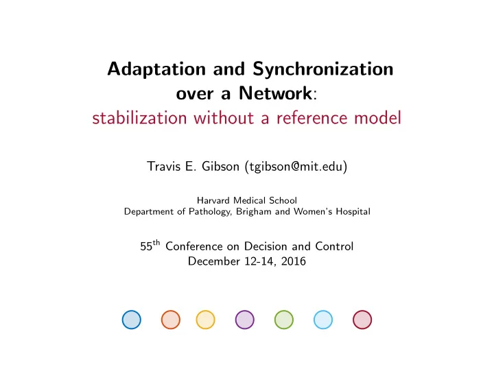
Adaptation and Synchronization over a Network : stabilization without a reference model Travis E. Gibson (tgibson@mit.edu) Harvard Medical School Department of Pathology, Brigham and Women’s Hospital 55 th Conference on Decision and Control December 12-14, 2016

Problem Statement Adaptive Systems Network Consensus Error System Generation Parameter Adaptation Consensus Error ◮ How do we achieve consensus and learning without a reference model? ◮ Can synchronous inputs enhance adaptation? 2 / 22

Introduction and Outline ◮ Synchronization can hurt learning ◮ Example of two unstable systems (builds on Narendra’s recent work) ◮ Synchronization and Learning in Networks ◮ Results Using Graph Theory ◮ Concrete connections to classic adaptive control (if time allows) 3 / 22

Synchronization vs. Learning: Tradeoffs 4 / 22

Two systems stabilizing each other Consider two unstable systems [Narendra and Harshangi (2014)] Σ 1 : x 1 ( t ) = a 1 ( t ) x 1 ( t ) + u 1 ( t ) ˙ Σ 2 : x 2 ( t ) = a 2 ( t ) x 2 ( t ) + u 2 ( t ) ˙ Update laws a 1 ( t ) = − x 1 ( t ) e ( t ) ˙ a 1 (0) > 0 a 2 ( t ) = x 2 ( t ) e ( t ) ˙ a 2 (0) > 0 with e = x 1 − x 2 . No Input 20 3 2 x 1 a 1 15 x 2 a 2 u 1 = 0 1 x 1 , x 2 a 1 , a 2 10 0 u 2 = 0 -1 5 -2 0 -3 0 5 10 0 5 10 t t 5 / 22

Synchronization Hurts Learning Synchronous Input × 10 5 12 2 u 1 = − e 10 x 1 a 1 1.8 x 2 a 2 8 u 2 = + e 1.6 x 1 , x 2 a 1 , a 2 6 1.4 4 1.2 2 e = x 1 − x 2 0 1 0 5 10 0 5 10 t t Desynchronous Input 8 4 x 1 a 1 6 2 x 2 a 2 u 1 = + e 4 0 x 1 , x 2 a 1 , a 2 u 2 = − e 2 -2 0 -4 -2 -6 0 5 10 0 5 10 t t 6 / 22

Stability Results for Synchronous and Desynchronous Inputs Σ 1 : x 1 ( t ) = a 1 ( t ) x 1 ( t ) + u 1 ( t ) ˙ Σ 2 : x 2 ( t ) = a 2 ( t ) x 2 ( t ) + u 2 ( t ) ˙ a 1 ( t ) = − x 1 ( t ) e ( t ) ˙ a 2 ( t ) = x 2 ( t ) e ( t ) ˙ Theorem: Synchronous Inputs The dynamics above with synchronous inputs have a set of initial conditions with non-zero measure for which x 1 and x 2 tend to infinity while e ∈ L 2 ∩ L ∞ and e → 0 as t → ∞ . Furthermore, this set of initial conditions that are unstable is also unbounded. Theorem: Desynchronous Inputs The dynamics above with desynchronous inputs are stable for all a 1 (0) � = a 2 (0) 7 / 22

Synchronization and learning in networks 8 / 22

Graph Notation and Consensus v 1 v 4 Graph : G ( V , E ) Vertex Set : V = { v 1 , v 2 , . . . , v n } Edge Set : ( v i , v j ) ∈ E ⊂ V × V v 2 v 3 � 1 if ( v j , v i ) ∈ E Adjacency Matrix : [ A ] ij = 0 otherwise In-degree Laplacian : L ( G ) = D ( G ) − A ( G ) In-degree of Node i : [ D ] ii Consensus Problem � Σ i : x i = − ˙ ( x i − x j ) j ∈N in ( i ) Using Graph Notation x = [ x 1 , x 2 , . . . , x n ] T Σ : x = −L x, ˙ 9 / 22

Review: Sufficient Condition for Consensus Σ : x = −L x ˙ Theorem: (Olfati-Saber and Murray, 2004) For the dynamics above with G strongly connected it follows that lim t →∞ x ( t ) = ζ 1 , for some finite ζ ∈ R . If G is also balanced � n then ζ = 1 i =1 x i (0) , i.e. average consensus is reached. n strongly connected there is a walk between any two vertices in the network. balanced if the in-degree of each node is equal to its out-degree. ◮ Any strongly connected digraph can be balanced (Marshall and Olkin, 1968) . ◮ Distributed algorithms exist to balance a digraph (Dominguez-Garcia and Hadjicostis, 2013) . 10 / 22

Return to Adaptive Stabilization Consider a set of n possibly unstable systems Σ i x i ( t ) = a i x i + θ i ( t ) x ˙ Update Law ˙ � θ i = − x i ( x i − x j ) j ∈N in ( i ) Compact form Σ : x = Ax + diag( θ ) x ˙ [ A ] ii = a i ˙ θ = [ θ 1 , θ 2 , . . . , θ n ] T θ = − x ◦ L x 11 / 22

Stabilization over Strongly Connected Graphs x = Ax + diag( θ ) x ˙ ˙ θ = − x ◦ L x Theorem For the dynamics above with G a strongly connected digraph, and all the a i + θ i (0) not identical it follows that lim t →∞ x ( t ) = 0 . ◮ G is strongly connected = ⇒ λ i ( L ) ∈ closed right-half plane of C . ◮ −L is Metzler = ∃ Diagonal D > 0 s.t. −L T D − D L ≤ 0 . ⇒ ◮ Non-increasing function � t n n � x T D L x d t + � [ D ] ii θ i ( t ) = − [ D ] ii θ i (0) 0 i =1 i =1 � t n = − 1 x T ( D L + L T D ) x d t + � [ D ] ii θ i (0) . 2 0 i =1 ◮ L 1 = 0 = ⇒ 1 T ( D L + L T D ) 1 = 0 . ◮ ∃ κ � λ 2 ( D L + L T D ) > 0 = x T x d t + � ⇒ � i [ D ] ii θ i ( t ) ≤ − κ � i θ i (0) when x / ∈ span( 1 ) . 12 / 22

Stabilization over Connected Graphs ◮ Any connected digraph can be partitioned into disjoint subsets called Strongly Connected Components (SCCs) where each subsets is a maximal strongly connected subgraph Condensed Graph Graph G SCC G root condensed nodes in red ◮ For any connected G the corresponding G SCC is a Directed Acyclic Graph ( DAG ) ◮ Every connected DAG contains a root node (not unique). 13 / 22

Stabilization over Connected Graphs Cont. x = Ax + diag( θ ) x ˙ ˙ θ = − x ◦ L x Theorem For the dynamics above with the adaptation occurring over a con- nected graph G such that a root can be chosen in G SCC that is a condensed node, then lim t →∞ x ( t ) = 0 ◮ The root is a strongly connected subgraph (thus stabilizes itself) ◮ All information flowing over G decimates from a stable SCC. ◮ Stability of each SCC then follows from the hierarchical structure of the DAG. G SCC 14 / 22

Stabilization over Connected Graphs: Example of Necessity This node can never stabilize if initially unstable 15 / 22

Consensus and Leaning Bring everything together as a layered architecture ◮ The communication graph is G ◮ G a is the adaptation graph and is constrained by the communication in G ◮ G s is the synchronization graph and is similarly constrained G G a G s (Doyle and Csete, 2011), (Alderson and Doyle, 2010) 16 / 22

Adaptive Stabilization over a Network Σ : x = Ax + diag( θ ) x ˙ ˙ θ = − x ◦ L a x G a = 1.5 1 1 0 0.5 -1 x i θ i 0 -2 -0.5 -3 -1 -4 0 5 10 0 5 10 t t 17 / 22

Adaptive Stabilization and Desynchronous Input Σ : x = Ax + L s x + diag( θ ) x ˙ ˙ θ = − Γ x ◦ L a x G a = G s = 1 2 0.5 0 0 x i θ i -2 -0.5 -4 -1 -1.5 -6 0 5 10 0 5 10 t t 18 / 22

Summary Borrowing from Narendra , Murray , and My Thesis , we have ◮ Found that synchronization can hurt learning. ◮ As always context is important ◮ What about other learning paradigms, i.e. Jadbabaie’s work or the broader Machine Learning literature Bibliography Alderson, D. L and J. C Doyle. 2010. Contrasting views of complexity and their implications for network-centric infrastructures , Systems, Man and Cybernetics, Part A: Systems and Humans, IEEE Transactions on 40 , no. 4, 839–852. Dominguez-Garcia, A. D. and C. N. Hadjicostis. 2013. Distributed matrix scaling and application to average consensus in directed graphs , Automatic Control, IEEE Transactions on 58 , no. 3, 667–681. Doyle, J. C. and M. Csete. 2011. Architecture, constraints, and behavior , Proceedings of the National Academy of Sciences 108 , no. Supplement 3, 15624–15630. Marshall, A. W and I. Olkin. 1968. Scaling of matrices to achieve specified row and column sums , Numerische Mathematik 12 , no. 1, 83–90. Narendra, K. S. and P. Harshangi. 2014. Unstable systems stabilizing each other through adaptation , American Control Conference, pp. 7–12. Olfati-Saber, R. and R. M Murray. 2004. Consensus problems in networks of agents with switching topology and time-delays , Automatic Control, IEEE Transactions on 49 , no. 9, 1520–1533. 19 / 22

C losed-loop R eference M odel (CRM) feedback gain ℓ x m Reference Model - � e r x � Plant θ ( t ) γ learning rate 20 / 22

How does CRM Help? reference: x m plant: x Classic Open-loop Reference Model (ORM) Adaptive ( ℓ = 0 ) ◮ The reference model does not adjust to any outside factors t reference: x m plant: x Closed-loop Reference Model (CRM) Adaptive ◮ The reference model adjusts to rapidly reduce the model following error e = x − x m t 21 / 22

CRM Simulation Examples 2.5 1 x m θ 2 x p k Parameter 0.5 1.5 State 0 γ = 10 1 -0.5 ℓ = 0 0.5 -1 0 0 10 20 30 0 10 20 30 t t 2.5 1 x o θ 2 m x m k Parameter 0.5 1.5 x p State 0 γ = 100 1 -0.5 ℓ = − 100 0.5 -1 0 0 10 20 30 0 10 20 30 t t 2.5 1 x o θ 2 m x m k Parameter 0.5 1.5 x p State 0 γ = 100 1 -0.5 ℓ = − 1000 0.5 -1 0 0 10 20 30 0 10 20 30 t t How do you choose γ and ℓ ? 22 / 22