A unified continuum mechanical approach for the computer age About - - PDF document

SLIDE 1

Mathematical Modeling of Flow, Heat Transfer, and Deformation

A unified continuum mechanical approach for the computer age

Hans Petter Langtangen Simula Research Laboratory and

• Dept. of Informatics

University of Oslo August 2004

– p. 1

About the course

About the course – p. 2

Overview

How this course differs from standard (continuum mechanical) modeling courses The two tracks of the course: application and theory Specification of required background

About the course – p. 3

Past and present

Traditional modeling Modern computational modeling

model formulation governed by available analytical solution techniques model formulation governed by numerical solution methods and available software tendency towards over-simplified models because of limited solution techniques more general models for phenomena of more industrial/scientific relevance

• ften sloppy treatment of initial and

boundary conditions numerics demands complete specification of initial-boundary value problems result as symbolic expressions result as visualizations

About the course – p. 4

What is modeling?

People mean different things by this term... Here: establishing a complete specification of the mathematical description for a physical phenomenon The term “complete specification” here means all input data required for applying a numerical method, i.e., a computer program to simulate the physical phenomenon Continuum mechanical modeling: model = partial differential equations (PDEs) + boundary and initial conditions

About the course – p. 5

Working style in this course

Find the basic governing equations and types of boundary conditions for the physical phenomon in question Note: physics, mechanics, geology++ books/people are often more concerned with the pheonoma and their explanations in terms of simple models than “full 3D models” (which we now want in the computer age) Find the relevant physical and mathematical assumptions that can be applied to reduce the complexity of the model Note: in the computer age we tend to reduce much less than in the paper-and-pencil age Imagine and argue for the expected qualitative behavior of a solution

About the course – p. 6

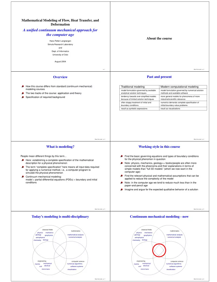
Today’s modeling is multi-disciplinary

engineering mechanical marine civil micro/nano electical classical fields physics mechanics geology astrophysics geophysics chemestry biology mathematics mathematical analysis numerical analysis computer science numerical algorithms software systems visualization

About the course – p. 7

Continuum mechanical modeling - now

engineering mechanical marine civil micro/nano electical classical fields physics mechanics geology astrophysics geophysics chemestry biology mathematics mathematical analysis numerical analysis computer science numerical algorithms software systems visualization

About the course – p. 8

SLIDE 2

Continuum mechanical modeling - classical

classical fields marine mathematics mathematical analysis mechanics physics engineering mechanical civil

About the course – p. 9

What you will learn

I have a physical phenomenon I want to simulate... Which program should I use? (i.e., what are the PDEs?) What is the complete specification of input data, i.e., boundary and initial conditions, coefficients in the PDEs etc. in my problem? Is the solution I get reasonable? Am I using the program correctly? (i.e., can I reproduce known solutions?) How do I debug a simulation with obviously wrong results? (i.e., how can I simplify and control?)

About the course – p. 10

Modeling implies approximation

“All models are wrong, but some models are useful” (George

• E. P

. Box) Models are useful even if the quantiative results are ridiculous, as long as the qualitative effects give insight The modeling approximation highly influences the choice of numerical approximations (i.e. methods) Approximation in the computer age differs from classical approximations

About the course – p. 11

Course: track (1)

The concept of stress Jump start: adapting the general heat transfer equation viscous fluid flow equation elasticity equation to various practical problems Formulation of (initial-) boundary value problems Emphasis on solving practical problems

About the course – p. 12

Prerequisites

Required background: broad experience with calculus, mathematical modeling of physical systems, interest in mathematics as a tool Advantageous background: introductory courses on fluid mechanics, familiarity with stress and strain

About the course – p. 13

Course: track (2)

(Euler/Lagrange description, strain) Mass, momentum, and energy balance Constitute laws: Newtonian fluids, generalized Newtonian fluids, linear elasticity, elasto-visco-plasticity, heat conduction etc. General models: 3D elasticity, Navier-Stokes, heat convection-diffusion Simplified models (potential flow, torsion, beams, gasdynamics, etc) Coupled models: flow, deformation and heat transfer

About the course – p. 14

Focus

Physical phenomenon → PDE model Generic PDEs with diverse application areas Derive (new) PDE models from basic principles Reduce models (i.e. remove terms) Formulate with computer in mind See visualizations of numerical solutions Solve and study simple problems analytically

About the course – p. 15

What we do not treat

Advanced continuum mechanics in the classical sense (go to the books!) The micro-physical basis of constitutive laws The (difficult) mathematics of constitutive laws Classical solution methods (“local tricks”) of certain continuum mechanical PDEs

About the course – p. 16

SLIDE 3

Twisting a rod (1)

An elastic cylinder is subject to a twisting moment. What is the stress state?

M M

twising moment twising moment

x y z L a

About the course – p. 17

Twisting a rod (2)

You can find a simple solution of this problem in any book on elasticity What if the cross section is more complicated? What is the relevant model now? (−∇2u = 2) How can I apply a 3D elasticity model?

About the course – p. 18

Flow around an obstacle (1)

• ✁

✁ ✁ ✂ ✂ ✂ ✄ ✄ ✄ ☎ ☎ ☎ ✆ ✆ ✆ ✝ ✝ ✝ ✞ ✞ ✞ ✟ ✟ ✟ ✠ ✠ ✠ ✡ ✡ ✡ ☛ ☛ ☛ ☞ ☞ ☞ ✌ ✌ ✌ ✍ ✍ ✍ ✎ ✎ ✎ ✏ ✏ ✏ ✑ ✑ ✑

How can I model this flow? (PDEs? BCs?)

About the course – p. 19

Flow around an obstacle (2)

The Navier-Stokes equations? ̺(v,t + (v · ∇)v) = −∇p + µ∇2v + ̺b ∇ · v = 0 But in fluid flow one also has the simple PDE ∇2φ = 0 What are the BCs? What about the common stream function model: ∇2ψ = vorticity What are the BCs now? Can I apply all three models?

About the course – p. 20

Flow in layered porous media (1)

✒ ✒ ✒ ✒ ✒ ✒ ✒ ✒ ✒ ✒ ✒ ✒ ✒ ✒ ✒ ✒ ✒ ✒ ✒ ✒ ✒ ✒ ✒ ✒ ✒ ✒ ✒ ✒ ✒ ✒ ✒ ✒ ✒ ✒ ✒ ✒ ✓ ✓ ✓ ✓ ✓ ✓ ✓ ✓ ✓ ✓ ✓ ✓ ✓ ✓ ✓ ✓ ✓ ✓ ✓ ✓ ✓ ✓ ✓ ✓ ✓ ✓ ✓ ✓ ✓ ✓ ✓ ✓ ✓ ✓ ✓ ✓ ✔ ✔ ✔ ✔ ✔ ✔ ✔ ✔ ✔ ✔ ✔ ✔ ✔ ✔ ✔ ✔ ✔ ✔ ✔ ✔ ✔ ✔ ✔ ✔ ✔ ✔ ✔ ✔ ✔ ✔ ✔ ✔ ✔ ✔ ✔ ✔ ✕ ✕ ✕ ✕ ✕ ✕ ✕ ✕ ✕ ✕ ✕ ✕ ✕ ✕ ✕ ✕ ✕ ✕ ✕ ✕ ✕ ✕ ✕ ✕ ✕ ✕ ✕ ✕ ✕ ✕ ✕ ✕ ✕ ✕ ✕ ✕

k k k k k

1 2 3 4 5

v prescribed Incompressible fluid; inflow velocity vin known

About the course – p. 21

Flow in layered porous media (2)

Some (textbooks) will attack the problem as a 1D flow problem and set up some flux continuity requirements... What if we consider

✖ ✖ ✖ ✖ ✖ ✖ ✖ ✖ ✖ ✖ ✖ ✖ ✖ ✖ ✖ ✖ ✖ ✖ ✖ ✖ ✖ ✖ ✖ ✖ ✖ ✖ ✖ ✖ ✖ ✖ ✖ ✖ ✖ ✖ ✖ ✖ ✖ ✖ ✖ ✖ ✖ ✖ ✖ ✖ ✖ ✖ ✖ ✖ ✖ ✖ ✖ ✖ ✖ ✖ ✖ ✖ ✖ ✖ ✖ ✖ ✖ ✖ ✖ ✖ ✖ ✖ ✖ ✖ ✖ ✖ ✖ ✖ ✖ ✖ ✗ ✗ ✗ ✗ ✗ ✗ ✗ ✗ ✗ ✗ ✗ ✗ ✗ ✗ ✗ ✗ ✗ ✗ ✗ ✗ ✗ ✗ ✗ ✗ ✗ ✗ ✗ ✗ ✗ ✗ ✗ ✗ ✗ ✗ ✗ ✗ ✗ ✗ ✗ ✗ ✗ ✗ ✗ ✗ ✗ ✗ ✗ ✗ ✗ ✗ ✗ ✗ ✗ ✗ ✗ ✗ ✗ ✗ ✗ ✗ ✗ ✗ ✗ ✗ ✗ ✗ ✗ ✗ ✗ ✗ ✗ ✗ ✘ ✘ ✘ ✘ ✘ ✘ ✘ ✘ ✘ ✘ ✘ ✘ ✘ ✘ ✘ ✘ ✘ ✘ ✘ ✘ ✘ ✘ ✘ ✘ ✘ ✘ ✘ ✘ ✘ ✘ ✘ ✘ ✘ ✘ ✘ ✘ ✘ ✘ ✘ ✘ ✘ ✘ ✘ ✘ ✘ ✘ ✘ ✘ ✘ ✘ ✘ ✘ ✘ ✘ ✘ ✘ ✘ ✘ ✘ ✘ ✘ ✘ ✘ ✘ ✘ ✘ ✘ ✘ ✘ ✘ ✘ ✘ ✘ ✘ ✙ ✙ ✙ ✙ ✙ ✙ ✙ ✙ ✙ ✙ ✙ ✙ ✙ ✙ ✙ ✙ ✙ ✙ ✙ ✙ ✙ ✙ ✙ ✙ ✙ ✙ ✙ ✙ ✙ ✙ ✙ ✙ ✙ ✙ ✙ ✙ ✙ ✙ ✙ ✙ ✙ ✙ ✙ ✙ ✙ ✙ ✙ ✙ ✙ ✙ ✙ ✙ ✙ ✙ ✙ ✙ ✙ ✙ ✙ ✙ ✙ ✙ ✙ ✙ ✙ ✙ ✙ ✙ ✙ ✙ ✙ ✙

k k k k k

1 2 3 4 5

p=const p=const

This course: view the world through 3D general models, then

About the course – p. 22

After the course you may say...

Now I see why the Poisson equation is so important Now I see the close relationship between potential flow, gasdynamics and the Navier-Stokes equations Now I see the (mathematical) similarities between elasticity and fluid flow Now I know how a 1D phenomena can be simulated by a 3D program Now I realize how models/PDEs from different fields are coupled I didn’t know that continuum modeling was that simple!

About the course – p. 23

Basic continuum mechanics

Basic continuum mechanics – p. 24

SLIDE 4

Notation

Notation – p. 25

Scalar, vector and tensor

vectors: v, vi, {vi} vi means either comp. no. i or the complete vector tensors: σ, σij, {σij} scalars: ̺ spatial point: r or x time: t

Notation – p. 26

Index notation (1)

Derivatives: u,t ≡ ∂u ∂t , vi,t ≡ ∂vi ∂t Summation convention: ukvk ≡

3

• k=1

ukvk sum over repeated index Example: σij,j ≡

3

• j=1

∂σij ∂xj divergence ofσij

Notation – p. 27

Index notation (2)

Kronecker delta: δij =

• 1,

i = j 0, i = j

• r

I =    1 1 1    Example: δijvj ≡

3

• j=1

δijvj = δi1v1 + δi2v1 + δi3v3 Only one of the δij factors can be nonzero, so if i = 3 we get δ3jvj = v3, i.e., in general δijvj = vi

Notation – p. 28

Representations of vectors

In a specific coordinate system we can evaluate a vector, using its coordinates, i.e. the coefficients in the vector’s expression, as a sum

• f scaled unit vectors

Vector v: v = (v1, v2, v3) v = v1i1 + v2i2 + v3i3 v = vkik v = (vx, vy, vz) v = vxi + vyj + vzk v = vrir + vθiθ (polar)

Notation – p. 29

Representation of tensors (1)

In a specific coordinate system we can evaluate a tensor, using its coordinates, i.e. the coefficients in the tensor’s expression as a sum of scaled unit tensors A =    A11 A12 A13 A21 A22 A23 A31 A32 A33    = A11    1    + A12    1    + · · · = A11ii + A12ij + · · ·

Notation – p. 30

Representation of tensors (2)

A =    Axx Axy Axz Ayx Ayy Ayz Azx Azy Azz    A = Axxii + Axyij + · · · + Azzkk A = A11i1i1 + A12i1i2 + · · · + A33i3i3 A = Aijiiij A = Arririr + Arθiriθ + · · · + Azrkir + · · ·

Notation – p. 31

Example (1)

What does σijnj mean? j is repeated, so we have a sum: σijnj =

3

• j=1

σijnj This is a matrix-vector product σ · n yielding a vector:    σxx σxy σxz σyx σyy σyz σzx σzy σzz       nx ny nz    =    sx sy sz    that is, σijnj = si

Notation – p. 32

SLIDE 5

Example (2)

What does σijni mean? Sum over repeated index: σijni =

3

• i=1

σijni =

3

• i=1

niσij This is a vector-matrix product nT σ or n · σ or

• nx

ny nz

• 

  σxx σxy σxz σyx σyy σyz σzx σzy σzz    =

• sx

sy sz

• that is: σijni = sj

Notation – p. 33

Esthetics

When having an expression on the form σijni = sj some prefer to use i as subscript for a vector result (si) This can be obtained by switching indices (i ↔ j): σjinj = njσji = si Be prepared for mathematical steps consisting of a change of letters in subscripts, just to make the end result more esthetic

Notation – p. 34

Formulas that should be recognized

Tensor-vector product: σijnj Vector-tensor product: niσij or σjinj Inner tensor-tensor product: σijσij Standard tensor-tensor product: σikτkj Outer (dyadic) product: aibj

Handy rule: σijnj has sum over j, hence one index survives and the result is a vector.

⇒ count surviving indices!

Notation – p. 35

Properties of the Kronecker delta

Index contraction: viδij = vj Index contraction: σijδjk = σik Summation convention: δii = 3 No summation convention: δii = 1 Relevant example: (uk,kδij),j = (uk,k),i = uk,ki The corresponding vector notation reads ∇ · [(∇ · u)I] = ∇(∇ · u)

Notation – p. 36

Yet another index/notation example

Interpret (ui,j),j: (ui,j),j =

• j

∂ ∂xj ∂ui ∂xj

• = ui,jj

=

• j

∂2ui ∂x2

j

= ∇2ui What about (µui,j),j for non-const. µ? (µui,j),j =

• j

∂ ∂xj

• µ ∂ui

∂xj

• = ∇ · [µ∇ui]

Notation – p. 37

Difficulties with the new notation?

Write out in matrix form!

• ∂

∂x ∂ ∂y ∂ ∂z

• 

  ∇ · u ∇ · u ∇ · u    =   

∂ ∂x∇ · u ∂ ∂y∇ · u ∂ ∂z∇ · u

   = ∇(∇ · u)

Notation – p. 38

Continuous media and molecules/atoms

Paradox: density ̺(r, t) is a continuous field, but what about the void space between molecules? Solution: ̺(r, t) is an averaged quantity, averaged over a volume containing a large number of molecules

Notation – p. 39

Interpretation of density

Pick a small volume ∆V and compute its mass ∆M Define the average density ̺(a) = ∆M/∆V Then define ̺(r, t) =

• lim∆V →0 ∆M/∆V

(mathematically) ̺(a), r is centroid of ∆V (physically) ⇒ ̺(r, t) is the average density in a small volume, often called continuum particle, around the point r at time t

Notation – p. 40

SLIDE 6

Interpretation of velocity

Pick a small volume (continuum particle) and compute the average of the velocities of all molecules inside this volume (particle): v(a) Then define v(r, t) =

• lim∆V →0 v(a)

(mathematically) v(a), r is centroid of ∆V (physically) ⇒ v(r, t) is the average velocity of the molecules inside a continuum particle with centroid at the point r at time t

Notation – p. 41

Fundamental quantities

̺(x, t): density v(x, t): velocity u(x, t): displacement T(x, t): temperature σ(x, t): stress tensor p(x, t): pressure Any f(x, t) means f evaluated for a (mathematically infinitesimal) continuum particle at time t and with centroid at point x

Notation – p. 42

Cylindrical coordinates (1)

r, θ, z) ( θ y θ i ir r x r, θ, z) ( r θ x y rsin rcos θ θ

(r, θ, z) ↔ (x, y, z) mapping: x = r cos θ y = r sin θ z = z Unit vectors: ir, iθ, k

Notation – p. 43

Cylindrical coordinates (2)

r, θ, z) ( θ y θ i ir r x r, θ, z) ( r θ x y rsin rcos θ θ

Unit vectors expressed by constant unit vectors: ir = cos θ i + sin θ j, iθ = − sin θ i + cos θ j Observe that ir and iθ vary with θ! ∂ir ∂θ = iθ, ∂iθ ∂θ = −ir Vector of a point: r = r ir + z k (notice: ir = ir(θ), hence r depends on θ too!)

Notation – p. 44

Circular motion (1)

θ x y r

A continuum particle moves in a circular path r: position of the particle r = rir with r constant (but θ and therefore ir vary with time)

Notation – p. 45

Circular motion (2)

θ x y r

Velocity of the particle: v = dr dt = d dt (rir) = rdir dt = ∂ir ∂θ dθ dt = r ˙ θiθ ⇒ v, directed along iθ, is tangent to the path (reasonable!) ˙ θ is the angular velocity

Notation – p. 46

Circular motion (3)

Acceleration of the particle: a = dv dt = r¨ θiθ + r ˙ θ(−ir) ˙ θir = r¨ θiθ − r ˙ θ2ir = acceleration along the path + centripetal acceleration Common case: constant angular velocity ˙ θ ⇒ only centrepetal acceleration

Notation – p. 47

Abbreviations

PDE = partial differential equation BC = boundary condition IC = initial condition BVP = boundary-value problem (= PDE in 1D with BC)

Notation – p. 48

SLIDE 7

Forces and stress

Forces and stress – p. 49

Body forces

body

• r

internal part of body b

Body forces b are “distant” forces acting in each point of the body Example: gravity b = g Example: centrifugal force b = ω × ω × r Total force: B =

• body

̺b dV

Forces and stress – p. 50

Gravity force on a brick

Problem 1: find the total gravity force on a brick W × H × D. Solution: B =

• V

̺g dV = ̺g

• V

dV = ̺gWHD = Mg, M = ̺WHD

Forces and stress – p. 51

Centrifugal force on a disk

Problem 2: find the total centrifugal force on a disk rotating with angular velocity ω = ωk around its center. Solution: B =

• V

̺ω × ω × r dV =

• V

̺ω2r dV, r = rir = r(cos θi + sin θj) = ̺ω2 L 2π a r(cos θi + sin θj)rdrdθdz =

Forces and stress – p. 52

Surface forces

s

body

• r

internal part of body

Distributed along the surface of a body or of an internal part of a body Stress = force per unit area, s(x, t) Total force: S(x, t) =

• surface

s(x, t)dA

Forces and stress – p. 53

Surface force on a sphere (1)

p(z)=az+b R (p,q)

What is the total force on the submerged sphere? S(t) =

• surface

s(x, t)dA, s(x, t) = −p(z)n = (az + b)(−n)

Forces and stress – p. 54

Surface force on a sphere (2)

S(t) =

• surface

(az + b)(−n)dA Spherical coordinates: x = p + r cos θ sin φ z = q + r cos φ y = 0 + r sin θ sin φ dA = R2 sin φ dθdφ Normal vector: n = ir = i cos θ sin φ + k cos φ + j sin θ sin φ

Forces and stress – p. 55

Surface force on a sphere (3)

S(t) = π 2π (a(q + R cos φ) + b) ×[−i cos θ sin φ − k cos φ − j sin θ sin φ]R2 sin φdθdφ = −2π π R2(a(q + R cos φ) + b) cos φ sin φdφ k = −a4 3πR3 k = Mgk, M = 4 3̺πR3 a < 0: force directed upwards (reasonable!)

Forces and stress – p. 56

SLIDE 8

Archimedes law (1)

Pressure force on a body: S =

• surface

p(−n)dA Gauss theorem (≈ “divergence theorem”):

• surface

p(−n)dA = −

• body

∇p dV ⇒ S = −

• V

∇p dV, V = body

Forces and stress – p. 57

Archimedes law (2)

Pressure in fluid at rest: p = p0 − ̺g(z − z0), ∇p = −̺gk Using this in S = −

• V

∇p dV, V = body gives S =

• V

̺gk dV = ̺gV k = Mg k The pressure on a body equals the mass of the displaced water, M = ̺V , times gravity and is directed upwards

Forces and stress – p. 58

The stress vector

Stress is force per unit area (vector) The stress vector depends on the orientation of the area That is, the stress at a point on a surface depends on the location of the point (on the surface) and on the orientation of the surface at that point

Forces and stress – p. 59

Stress in a rod

• ✁

✁ ✁ ✁ ✁ ✁ ✂ ✂ ✂ ✂ ✂ ✂ ✄ ✄ ✄ ✄ ✄ ✄ ☎ ☎ ☎ ☎ ☎ ☎ ✆ ✆ ✆ ✆ ✆ ✆ ✝ ✝ ✝ ✝ ✝ ✝ ✞ ✞ ✞ ✞ ✞ ✞ ✟ ✟ ✟ ✟ ✟ ✟ ✠ ✠ ✠ ✠ ✠ ✠

F F F F F/2 F/2 F/2 F/2

Forces and stress – p. 60

Observations

The stress at the bullet point was in one case F/A (A: area) and in another case 0! “Stress” means stress at a point on a surface The surface orientation (normal vector n) is needed for stress vector computations

Forces and stress – p. 61

Stress vector computation

The stress vector depends on space, time and the orientation (unit

• utward normal vector n) of the surface on which the stress vector

acts Notation: s(r, t; n) (s varies in R7, i.e., with 7 parameters!) Cauchy’s 1. law: si(r, t; n) = nj(r, t)σji(r, t)

• r

s(r, t; n) = n(r, t) · σ(r, t) (⇒ s has a simple (linear) dependence on n)

Forces and stress – p. 62

The stress tensor

The quantity σ or σij in Cauchy’s 1. law is called the stress tensor σ contains 9 entries: σ =    σxx σxy σxz σyx σyy σyz σzx σzy σzz    The entries have a physical interpretation, but represent mainly ingredients in a tool (Cauchy’s 1. law) for computing the stress vector at an arbitrary surface

Forces and stress – p. 63

Interpretation of stress tensor entries

The interpretation of the stress tensor entries follows from Cauchy’s

• 1. law:

i · σ = stress vector on plane x = const i · σ = σxxi + σxyj + σxzk ⇒ σxx is normal stress on a plane x = const ⇒ σxy is shear stress in y direction on a plane x = const ⇒ σxz is shear stress in z direction on a plane x = const

Forces and stress – p. 64

SLIDE 9

Stress tensor in a rod (1)

F F

Uni-axial tension force How can we find the stress tensor in this case? General approach: solve the governing PDE with boundary conditions (possible even analytically!) Or: use physical reasoning to guess at a stress tensor (usually difficult, but possible in this case)

Forces and stress – p. 65

Stress tensor in a rod (2)

Cutting the body along coordinate planes (x = const, y = const, z = const)

• ✁

✁ ✁ ✁ ✁ ✁ ✂ ✂ ✂ ✂ ✂ ✂ ✄ ✄ ✄ ✄ ✄ ✄ ☎ ☎ ☎ ☎ ☎ ☎ ✆ ✆ ✆ ✆ ✆ ✆ ✝ ✝ ✝ ✝ ✝ ✝ ✞ ✞ ✞ ✞ ✞ ✞ ✟ ✟ ✟ ✟ ✟ ✟ ✠ ✠ ✠ ✠ ✠ ✠

F F F F F/2 F/2 F/2 F/2

suggests σ =    F/A   

Forces and stress – p. 66

Stress tensor in a rod (3)

How can we know that this guess is correct? Physical reasoning indicates such a stress tensor, but only the solution of a full model for elastic deformation can tell if our assumption of σ is correct Classically, such guesses based on physical reasoning were required to treat the problem analytically Today, such guesses are crucial to assess whether numerical results are reasonable

Forces and stress – p. 67

More on Cauchy’s laws

The stress tensor σij is all the information we need to find the stress

• n an arbitrary surface

Derivation of Cauchy’s 1. law: Study the force equilibrium of a tetrahedron Cauchy’s 2. law: σij = σji (symmetric tensor) derived from moment equilibrium of an arbitrary volume With the 2. law, we can rewrite the 1. law: si = njσji = σijnj

• r

s = n · σ = σ · n

Forces and stress – p. 68

Stress and density vs. mass and force?

Force (mass) depends on the size of the surface (volume) ⇒ Inconvenient in a continuous medium (okay for rigid body dynamics) Stress (density) has meaning at a point, and force (mass) is readily

• btained by integrating over the surface (volume)

force =

• surface

sdA, mass =

• volume

̺ dV

Forces and stress – p. 69

Normal and shear stress

n T s N

Normal stress: σN = s · n (= n · σ · n) Normal stress vector: N = σNn = (s · n)n Tangential/shear stress vector: T = s − N Tangential/shear stress: σT = ||T ||

Forces and stress – p. 70

Stress in a rod (1)

Consider

φ n F F

Stress tensor: σ =    F/A    How can we compute the stress vector on the inclined plane?

Forces and stress – p. 71

Stress in a rod (2)

We use Cauchy’s 1. law, as always, for computing a stress vector: s = σ · n Normal vector on the plane: n = cos φi + sin φj Applying Cauchy’s 1. law: s =    F/A       cos φ sin φ    = F A cos φ    1   

Forces and stress – p. 72

SLIDE 10

Stress in a rod (3)

s = F A cos φi, n = cos φi + sin φj Normal stress: σN = s · n = F A cos2 φ, N = F A cos2 φ n Shear stress: T = s − N = (F/A) cos φ(sin2 φ, − cos φ sin φ, 0)T )

Forces and stress – p. 73

Stress in a rod (4)

Suppose we are interested in the failure of the material Possible failure criterion I: max σN > C (max σN appears for φ = 0 ⇒ F/A > C) Possible failure criterion II: max σT > D Can find max σN and max σT by optimizing the expressions with respect to θ Formulas of general validity exist for maximum normal and shear stress, which are easier to use Such formulas require knowledge of principal stresses

Forces and stress – p. 74

Principal stresses/directions (1)

Definition: Orientation (n) of surfaces with normal stress only In mathematical terms: s = λn ⇔ (σ − λI) · n = 0 solve for n and λ Standard eigenvalue problem! Principal stresses = eigenvalues σI ≥ σII ≥ σIII (ordered!) Principal directions = eigenvectors n(I), n(II), n(III)

Forces and stress – p. 75

Principal stresses/directions (2)

What are the applications of principal stresses and directions? Main application: max/min normal/shear stresses for use in design (fracture, yield) criteria Symmetric, real σ ensures three real eigenvalues and three

• rthogonal eigenvectors

Forces and stress – p. 76

Max/min normal and shear stress

Find the surface orientations that lead to extreme normal and shear stress values at a point (r, t) Normal stress: σ2

N = ||N||2

Shear stress: σ2

T = ||T ||2

σ2

N and σ2 T are functions of n = (n1, n2, n3)

In mathematical terms: Find the extreme values of σ2

N(n1, n2, n3) and

σ2

T (n1, n2, n3) under the constraint n2 1 + n2 2 + n2 3 = 1

Constrained optimization problem Solution method: Lagrange multipliers

Forces and stress – p. 77

Principal steps of the solution process

Work with a diagonal σij, i.e., rotate the coordinate system such that the axes coincide with the principal directions and σ = diag(σI, σII, σIII) Trivial to optimize σ2

N

Straightforward to compute the extremes of σ2

T

Translate results to original coordinates ⇒ Nice exercise in multivariable optimization and linear algebra

Forces and stress – p. 78

Extreme normal stresses

Extreme values of σ2

N:

directions = principal directions values = principal values (Trivial calculations)

Forces and stress – p. 79

Extreme shear stresses

Extreme values of σ2

T :

Solution 1: along principal directions, but here σ2

T = 0 so this is a

minimum Solution 2 (maximum): σT = 1 2 |σI − σII| , n = 1 √ 2

• ±n(I) ± n(II)

σT = 1 2 |σII − σIII| , n = 1 √ 2

• ±n(II) ± n(III)

σT = 1 2 |σIII − σI| , n = 1 √ 2

• ±n(III) ± n(I)

The last line gives the max shear results if σI ≥ σII ≥ σIII

Forces and stress – p. 80

SLIDE 11

Why four directions?

There are four directions for each max shear candidate, e.g., σT = 1 2 |σIII − σI| , n = 1 √ 2

• ±n(III) ± n(I)

Why four directions? You can equally well use −n as n Because of the σij = σji symmetry, any shear stress on a surface with normal n will also be present as shear stress on an orthogonal surface, i.e., when σT acts on n = (n1, n2), σT also acts on (n1, −n2)

• r (−n1, n2)

Forces and stress – p. 81

Invariants

The characteristic polynomial of σ (i.e. det(σ − λI) = 0): λ3 + Iσλ2 + IIσλ − IIIσ = 0 Recall from linear algebra: λ is independent of the coordinate system (invariant) ⇒ The coefficients Iσ, IIσ and IIIσ must also be invariant The invariants of σ are Iσ, IIσ, IIIσ, these are used in many context in continuum mechanics, esp. in constitutive laws Formulas: Iσ = σii, IIσ = 1 2(σiiσjj − σijσij), IIIσ = det{σij}

Forces and stress – p. 82

Deviatoric tensors

One often works with the deviatoric stress tensor σ′ in continuum mechanics: deviatoric stress tensor = stress tensor – isotropic mean stress σ′

ij = σij − 1

3σkkδij

• r

σ′ = σ − 1 3trace(σ)I Note: σ′

kk = 0

−σkkδij is an isotropic pressure −σkkδij gives only normal stresses on all surfaces!

Forces and stress – p. 83

Pressure stress

A stress tensor on the form σij = −pδij represents an isotropic pressure Any surface is loaded with normal stress −p only Proof: stress at any surface = σijnj = −pδijnj = −pni i.e., directed in the normal direction, with magnitude p No shear stress can arise from such a stress state

Forces and stress – p. 84

Stress tensors in cylindrical coordinates

Cylindrical coordinates: x = r cos θ, y = r sin θ, z = z Tensor representations: A =    Arr Arθ Arz Aθr Aθθ Aθz Azr Azθ Azz    A = Arririr + Arθiriθ + Aθriθir + Arzirk + Azrkir + Aθθiθiθ + Aθziθk + Azθkiθ + Azzkk

Forces and stress – p. 85

Important observations

ir and iθ are functions of θ! ∂ir ∂θ = iθ, ∂iθ ∂θ = −ir ⇒ ∂ ∂θ (Arθiθir) = ∂Arθ ∂θ iθir + Arθ ∂iθ ∂θ

• ir + Arθiθ

∂ir ∂θ

• This has important implications for, e.g., ∇ · A and makes

computations in cylindrical coordinates more difficult than in Cartesian coordinates

Forces and stress – p. 86

Interpretation of stress components

A = Arririr + ArθArθiriθ + Aθriθir + Arzirk + Azrkir + Aθθiθiθ + Aθziθk + Azθkiθ) + Azzkk Does Arθ have a physical interpretation? Yes! The stress on a surface with ir as normal is ir · A = Arrir + Arθiθ + Arziz The θ-component of this stress vector is iθ · A · ir = Arθ ⇒ Arθ is the shear stress in θ-direction on a surface r = const Similar interpretations of the other components

Forces and stress – p. 87

Summary of basic models

Summary of basic models – p. 88

SLIDE 12

Current philosophy

Jump into the simplest full mathematical models for heat transfer, viscous flow and elastic deformations Study some simple examples on applying the models to physical problems Solve exercises Later: learn how the full models are derived, learn how to derive new models for extended problems

Summary of basic models – p. 89

What “solve” means

“Solve” in this course consists of two steps: Formulate a simplified version of the full mathematical models, adapted to a specific problem (omitting terms etc.) (if the simplified model is simple enough) find an analytical solution Interpretation step: Get insight from the analytical solution Study a numerical solution (visualizations)

Summary of basic models – p. 90

About analytical solutions

Traditionally, mechanics courses have only addressed problems for which one can find analytical solutions (or insight) There is much to learn from simple analytical solutions Analytical solutions play a key role in testing numerical software In this course we will look at all types of problems; if not an analytical solution can be found, the problem can be treated by numerical methods Numerical methods are beyond the scope of the course, but the results, in terms of visualizations, are not!

Summary of basic models – p. 91

Adapting a model to a problem

List all assumptions and their implications Omit time-dependent terms? Reduce dimensions (3D to 1D f.ex.)? Special functional structure of the unknown? Omit other terms? Utilize symmetry? Scaling? Specify boundary conditions Specify initial conditions Arrive at a well-posed PDE problem

Summary of basic models – p. 92

Basic quantities in heat transfer

Primary interest: temperature T Secondary interest: heat flow ∝ ∇T Primary unknown in mathematical models: T(r, t), temperature of a continuum particle at r at time t T is governed by a linear scalar PDE Details appear later

Summary of basic models – p. 93

Basic quantities in elasticity

Primary interest: stress tensor σ (σ enters design formulas, fracture criteria, reliability estimates etc.) Secondary interest: deformation field u Primary unknown in mathematical models: u(r, t), displacement of a solid particle at r at time t u is governed by a linear vector PDE σ is given by the derivatives of u Details appear later

Summary of basic models – p. 94

Basic quantities in viscous flow

Primary interest: velocity v, pressure p Secondary interest: stress tensor σ (e.g. integrated to forces on bodies in the flow) Primary unknowns in mathematical models: v(r, t), velocity of a fluid particle at r at time t p(r, t), pressure at r at time t v and p are governed by the Navier-Stokes equations (a coupled set

• f nonlinear vector PDEs)

σ is given by the derivatives of v Details appear later

Summary of basic models – p. 95

Summary of heat transfer

Summary of heat transfer – p. 96

SLIDE 13

Heat transfer in solids; PDE

Governing PDE in solids: ̺cT,t = (kT,j),j

• r alternatively

̺cT,t = ∇ · (k∇T) Origin: 1st law of thermodynamics ̺: density, c: heat capacity, k: heat conduction (̺, c and k can vary throughout a heterogeneous medium) Solve for the temperature T(r, t) Heat flow: q = −k∇T i.e. qi = −kT,i

Summary of heat transfer – p. 97

Heat transfer in fluids; PDE

Governing PDE in fluids: ̺c(T,t + vjT,j) = kT,jj

• r alternatively

̺c(T,t + v · ∇T) = k∇2T v: fluid velocity Solve for the temperature T(r, t) Heat flow: q = −k∇T i.e. qi = −kT,i Difference between PDE in solids and fluids: extra transport term (v · ∇T) and constant k in fluids

Summary of heat transfer – p. 98

Heat transfer; IC and BCs

If we have a time-dependent problem (T,t = 0), we must specify T initially: T(xj, 0) i.e. T(r, 0) Possible types of boundary conditions: T prescribed −k∂T/∂n ≡ −k∇T · n (heat flux) prescribed −k∂T/∂n = α(T − T0) (Newton’s cooling law; α is given, T0 is a temperature outside the domain) At each point on the boundary there must be one boundary condition

Summary of heat transfer – p. 99

Heat transfer; interface conditions

medium 1 medium 2 n

Two heat transfer conditions at any interface/surface: continuous temperature: T (1) = T (2) continuous heat flux: −k(1)T (1)

,n = −k(1)T (2) ,n

These conditions are automatically incorporated in the PDE with variable k; we only use them explicitly when solving separate problems in medium 1 and 2

Summary of heat transfer – p. 100

Heat transfer; illustration of BCs

k k2 1 T1 T0

Heat conduction in a solid built of two materials k =

• k1,

gray area k2,

• utside

Left black part of the boundary: T = T1 Right part of the boundary: T = T0 The rest of the boundary is insulated: −k∇T · n = −kT,n = 0

Summary of heat transfer – p. 101

Exercises

Extend the previous BC example to 3D Write out the heat transfer equation in a fluid in 3D: ̺c(∂T ∂t + vx ∂T ∂x + · · · ) = · · ·

Summary of heat transfer – p. 102

Summary of elasticity

Summary of elasticity – p. 103

Elastic solids; PDE

Governing PDE: Navier’s equation, ̺ui,tt = (λ + µ)uk,ki + µui,kk + ̺bi

• r alternatively

̺u,tt = (λ + µ)∇(∇ · u) + µ∇2u + ̺b Origin: Newton’s 2nd law b: body forces, ̺: density λ and µ are known parameters reflecting the elastic properties of the medium (here constant) Solve for the displacement u(r, t)

Summary of elasticity – p. 104

SLIDE 14

Elastic solids; PDE

If λ and µ varies (heterogeneous medium), the PDE becomes ̺u,tt = ∇[λ∇ · u] + ∇ · [µ(∇u + (∇u)T )] + ̺b The PDE is valid for small displacement and perfectly linearly elastic bodies Can extend this PDE with temperature effects (see later)

Summary of elasticity – p. 105

Elastic solids; stress

The quantity of major interest is the stress tensor, (usually) not the primary unknown in the PDE (displacement) The stress tensor is computed as a post-process, after u is found from the PDE model Hooke’s law relates the stress tensor to u: σij = λuk,kδij + µ(ui,j + uj,i)

• r alternatively

σ = λ∇ · uI + µ(∇u + (∇u)T )

Summary of elasticity – p. 106

Elastic solids; strain

A measure of the deformation of a solid body is the strain tensor: εij = 1 2(ui,j + uj,i)

• r alternatively:

ε = 1 2(∇u + (∇u)T ) Stress-strain relation: σ = λtrace(ε)I + 2µε

Summary of elasticity – p. 107

Elastic solids; ICs

If we have a time-dependent problem (ui,tt = 0), we must specify ui(xj, 0) i.e. u(r, 0) ui,t(xj, 0) i.e. u,t(r, 0) (The u,tt term in the PDE requires two ICs)

Summary of elasticity – p. 108

Elastic solids; BCs

Types of BCs in elasticity: Prescribed displacement u Prescribed stress vector σ · n In d space dimensions we need d conditions at every point of the boundary BCs can be mixed, e.g.,

• ne displacement and two stress components at a point (3D)

Rule: go through all boundary points and check that d conditions are specified!

Summary of elasticity – p. 109

Elastic solids; illustration of BCs

stress free boundary attached to wall force F x x2

1

Assumption: 2D problem ⇒ 2 BCs at every boundary point Wall: u1 = 0, u2 = 0 Right end: assuming F is uniformly distributed, s1 = F/A, s2 = 0 The rest: s1 = 0, s2 = 0

Summary of elasticity – p. 110

Remark on stress boundary conditions

If the elasticity problem is solved by finite element methods, it is natural to specify stress boundary conditions in terms of stress vector components For other solution methods (analytical, finite differences, ...), it is usually necessary to express the stresses in terms of the primary unknown (displacement) For example: s1 = 0 for finite elements λuk,k + 2µu1,1 = 0 otherwise s2 = 0 for finite elements λuk,k + 2µu2,2 = 0 otherwise Most common solution method is finite elements

Summary of elasticity – p. 111

Elastic solids; illustration of BCs

stress free boundary attached to wall force F x x2

1

Modification: at the wall, the body cannot move in x1-direction, but it can slide without friction in x2-direction This is the type of connection with the wall we must assume if the problem is to be solved analytically (since the shape is now independent of x1) Right end: assuming F is uniformly distributed, s1 = F/A, s2 = 0 The rest: s1 = 0, s2 = 0 Wall: u1 = 0, s2 = 0

Summary of elasticity – p. 112

SLIDE 15

Exercises

Extend the previous BC example to 3D Write out Navier’s equation in 2D (where 2D means u3 = 0 and ∂/∂x3 = 0): ̺∂2u1 ∂t2 = · · · ̺∂2u2 ∂t2 = · · ·

Summary of elasticity – p. 113

Elastic solids; interface conditions

medium 1 medium 2 n

Dynamic condition: continuous stress vector, σ(1) · n = σ(2) · n

• r expressed by the stress vector s = σ · n instead:

s(1) = s(2) Required by Newton’s 2nd law to prevent infinite acceleration of the boundary

Summary of elasticity – p. 114

Elastic solids; interface conditions

medium 1 medium 2 n

Kinematic condition: continuous displacement u(1) = u(2) That is, no cracks at the interface

Summary of elasticity – p. 115

Summary of viscous flow

Summary of viscous fl

• w – p. 116

Viscous fluids; PDE

Governing PDE: The Navier-Stokes equation (originates from Newton’s 2nd law) ̺(vi,t + vkvi,k) = −p,i + µvi,kk + ̺bi

• r alternatively

̺(v,t + (v · ∇)v) = −∇p + µ∇2v + ̺b plus the equation of continuity (originates from mass conservation) vk,k = 0

• r equivalently

∇ · v = 0

Summary of viscous fl

• w – p. 117

Viscous fluids; PDE

̺(v,t + (v · ∇)v) = −∇p + µ∇2v + ̺b ∇ · v = 0 µ: viscosity, ̺: density µ is constant (to be relaxed later) Solve for v(x, t) (velocity) and p(x, t) (pressure) The PDEs are valid for Newtonian and incompressible fluids The flow must be laminar (no chaotic turbulence) Remark: The PDEs describes turbulence, in fact, but requires an extremely fine grid for numerical solution – usually other equations are used for turbulent flow

Summary of viscous fl

• w – p. 118

Viscous fluids; stress

Sometimes the stress tensor is also of interest The stress tensor is found as a post-process after v and p are computed from the PDE model: σij = −pδij + µ(vi,j + vj,i)

• r alternatively

σ = −pI + µ(∇v + (∇v)T )

Summary of viscous fl

• w – p. 119

Viscous fluids; strain-rate

A measure of the deformation in a fluid is the strain-rate tensor: ˙ εij = 1 2(vi,j + vj,i)

• r alternatively:

˙ ε = 1 2(∇v + (∇v)T ) Stress-strain-rate relation: σ = −pI + 2µ ˙ ε

Summary of viscous fl

• w – p. 120

SLIDE 16

Viscous fluids; IC

If we have a time-dependent problem (vi,t = 0), we must specify one initial condition for v vi(xj, 0) i.e. v(r, 0) There is no initial condition for p

Summary of viscous fl

• w – p. 121

Viscous fluids; BCs

Types of BCs in viscous flow: Prescribed velocity v Prescribed stress vector s = σ · n (less used) Outflow condition: ∂v ∂n = 0 (no further change downstream) No “BCs” for p; p can only be specified (as a time series) at a point (!)

Summary of viscous fl

• w – p. 122

Viscous fluids; interface conditions

medium 1 medium 2 n

Dynamic condition: continuous stress vector, σ(1) · n = σ(2) · n

• r expressed by the stress vector s = σ · n instead:

s(1) = s(2) Required by Newton’s 2nd law to prevent infinite acceleration of the boundary

Summary of viscous fl

• w – p. 123

Viscous fluids; interface conditions

medium 1 medium 2 n

Kinematic condition: continuous velocity (no void space), v(1) = v(2)

Summary of viscous fl

• w – p. 124

Viscous fluids; how many BCs?

In d space dimensions we need d conditions at every point of the boundary Boundary conditions can be mixed, e.g., one velocity component and two normal derivatives can be prescribed Rule: go through all boundary points and check that d conditions are specified!

Summary of viscous fl

• w – p. 125

Viscous fluids; illustration of BCs

x x2

1

known velocity

• utflow

solid wall

Assumption: 2D problem (⇒ 2 BCs at each boundary point) Inlet: v1 specified, v2 = 0 Walls: v1 = 0, v2 = 0 (the wall is at rest) Outlet: v2 = 0, ∂v1/∂n = 0 Alternative outled conditions: ∂v2/∂n = 0, ∂v1/∂n = 0 (flexible!) or v1 prescribed as on the inlet boundary, v2 = 0 (not recommended – puts too many constraints on numerical solutions)

Summary of viscous fl

• w – p. 126

Exercises

Extend the previous BC example to 3D Write out Navier’s equation in 2D (where 2D means u3 = 0 and ∂/∂x3 = 0): ̺∂v1 ∂t = · · · ̺∂v2 ∂t = · · ·

Summary of viscous fl

• w – p. 127

Heat conduction example

Heat conduction example – p. 128

SLIDE 17

Heat conduction in a glacier

Problem: find the temperature (T) distribution and the heat flow through a glacier

glacier known temperature known heat flux z x H

Heat conduction example – p. 129

Basic equations in the model

This is heat transfer in a solid material ⇒ heat equation for T, ̺cT,t = ∇ · (k∇T) BCs depend on how many dimensions we include in the model, but at least we have basement z = 0: known heat flux −k∂T/∂n surface z = H: known temperature T

Heat conduction example – p. 130

Assumptions

Negligible air flow through the snow/ice (no coupling to flow equations) Stationary problem ⇒ T,t = 0 (⇒ no need for initial condition) Homogeneous medium (constant k, ̺ and c) The domain, coefficients and BCs do not change with x and y ⇒ ∂/∂x = 0, ∂/∂y = 0 Hence, T only varies with z: T = T(z)

Heat conduction example – p. 131

Simplifications

Basic assumptions from previous slide: T = T(z) Inserting T(z) in the heat conduction equation: kT ′′(z) = 0 The problem is now 1D (no need for boundary conditions as x, y → ±∞) Boundary condition at z = 0: kT ′(0) = −q (note: ∂T/∂n = −dT/dz) Boundary condition at z = H: T(H) = TH

Heat conduction example – p. 132

Summary: BVP

The original problem involving a three-dimensional PDE is now reduced to a two-point linear boundary value problem (BVP): T ′′(z) = T ′(0) = −q/k T(H) = TH Well-posed mathematical problem

Heat conduction example – p. 133

Solving the BVP

Straightforward integration (twice) of the PDE: T = Az + B A and B are determined from the boundary conditions T ′(0) = −q/k ⇒ A = −q/k and T(H) = TH ⇒ B = TH + qH/k Solution: T(z) = TH + q k(H − z) Heat flow: q = −k∇T = −kT ′(z)k = qk

Heat conduction example – p. 134

Extension to two materials

Assume the glacier has two layers with varying properties (here two values of k, but constant c and ̺):

known temperature known heat flux layer 1 layer 2 z x H

How can this problem be solved?

Heat conduction example – p. 135

Treatment of two materials

k is now a discontinuous function: k(z) =

• k1,

layer 1, H ≤ z ≤ c k2, layer 2, c < z ≤ 0 Alternative 1: solve for T with constant k in each domain and couple the solutions (typical approach for analytical calculations) Alternative 2: solve for T with a variable k (typical approach in numerical software)

Heat conduction example – p. 136

SLIDE 18

Alternative 1: two domains

In each layer, k is constant ⇒ apply the same solution procedure as when the problem contained only one layer T (1)(z) = A1z + B1, T (2)(z) = A2z + B2 Boundary conditions: T (1)(H) = TH, −k2 dT (2) dz (0) = q (only 2 conditions, need 4 for A1, A2, B1, B2)

Heat conduction example – p. 137

Alternative 1: interface BCs

We need two additional BCs Interface conditions (z = c): continuous temperature: T (1)(c) = T (2)(c) continuous heat flux: −k1T (1)

,z

= −k2T (2)

,z

(2+2=4 conditions in total) Linear 4 × 4 system for A1, A2, B1, B2

Heat conduction example – p. 138

Alternative 2: one domain

Now we work with k(z) and the simplified heat equation d dz

• k(z)dT

dz

• = 0 with − k2

dT dz

• z=0

= q, T(H) = TH Integrating once, dividing by k: T,z = C/k(z) Boundary condition at z = 0 determines C; C = k2q Integrating once more: T(z) = z k2q k(z)dz + D Determine D from T(H) = TH: k2q k2 c + k2q k1 (H − c) + D = TH Easier than alt. 1 in this case, but normally much more difficult in 2D and 3D

Heat conduction example – p. 139

Solution

Both approaches yield, of course, the same solution T(z) = TH − q(c − z) − k1 k2 q(H − c), 0 ≤ z ≤ c T(z) = TH − k2 k1 q(H − z), c < z ≤ H The flux: −k2T,z = −k2q, 0 ≤ z ≤ c −k1T,z = −k2q, c < z ≤ H Observe that the flux is constant The 2nd approach allows an arbitrary function k(z) > 0!

Heat conduction example – p. 140

Formulation as a 2D problem

known temperature known heat flux layer 1 layer 2 A B z x H

Now we have four sides Same BCs at the top and bottom as in the 1D problem But what about A and B?

Heat conduction example – p. 141

BC at vertical boundaries

We have assumed variation with z only → ∂T/∂x = 0 at A and B Derivatives are expressed as normal derivatives in BCs: ∂T/∂n = 0 at A and B

Heat conduction example – p. 142

Elasticity example

Elasticity example – p. 143

Stress and deformation in a glacier

Problem: find the deformation and the internal stresses in a glacier subjected to gravity forces

z x g elastic medium H no stress rigid bottom

Elasticity example – p. 144

SLIDE 19

Basic equations

This is elasticity Governing PDE is Navier’s vector equation for u: ̺u,tt = (λ + µ)∇(∇ · u) + µ∇2u + ̺b BCs depend on how many dimensions we include in the model, but at least we have z = 0: no displacement (u = 0) z = H: stress free boundary

Elasticity example – p. 145

Assumptions

Small deformations Stationary problem ⇒ ui,tt = 0 (⇒ no need for initial conditions) Homogeneous elastic medium (λ and µ const) Gravity is the main load: b = −gk or bi = −gδi3 No change of domain, coefficients or BCs in the x and y directions ⇒ ∂/∂x = 0, ∂/∂y = 0 Infinite layer (“walls at infinity”) ⇒ only a downward movement of the solid particles ⇒ u = w(z)k

Elasticity example – p. 146

Simplifications

Basic assumption from previous slide: u = w(z)k Inserting u = w(z)k in Navier’s equation gives ∇ · u = w,z(z), ∇2u = w,zz(z)k and the elasticity PDE reduces to w,zz(z) = ̺g λ + 2µ, 0 < z < H No need for boundary conditions as x, y → ±∞ as the problem is now 1D (such conditions are built-in in u; u1 = u2 = 0) Boundary condition at z = 0: w(0) = 0 Boundary condition at z = H: σ · k = 0

Elasticity example – p. 147

Stress tensor expressions

The BC at z = H: σ · k = 0 needs to be expressed in terms of w to get a mathematical model for w Need to express the stress tensor in terms of ‘w using σij = λuk,kδi,j + µ(ui,j + uj,i) Great simplifications with u = w(z)k: σ = w,z(z)    λ λ λ + 2µ    At z = H we then get {σij} · k = w,z(H)(λ + 2µ)k = 0 ⇒ w,z(H) = 0

Elasticity example – p. 148

Summary: BVP

The original three-dimensional problem, with three coupled linear partial differential equations, is now reduced to a two-point linear boundary value problem (BVP): w′′(z) = ̺g λ + 2µ, 0 < z < H w(0) = w′(H) = Well-posed mathematical problem

Elasticity example – p. 149

Solving the BVP

Straightforward integration (twice) of the PDE: w(z) = 1 2 ̺g λ + 2µz2 + Az + B A and B are determined from the boundary conditions: w(0) = 0 ⇒ B = 0 and w′(H) = 0 ⇒ A = −H ̺g λ + 2µ Solution: w(z) = ̺g λ + 2µ(z/2 − H)z

Elasticity example – p. 150

Finding the stresses

The stress tensor is derived as a post-process when the displacement is known (Hooke’s law) Here, with simplified displacement, σ = w,z(z)    λ λ λ + 2µ    that is, σ = ̺g λ + 2µ(z − H)diag(λ, λ, λ + 2µ) Observe: 0 > σxx = σyy > σzz σzz = ̺g(z − H) (reasonable!)

Elasticity example – p. 151

Max shear stress

From formulas: σ is diagonal ⇒ the principal values are on the diagonal and the principal directions are i, j and k Max shear stress: σT = ̺gµ λ + 2µ(H − z) Orientation of surfaces with max shear: 1 √ 2(±i ± k), 1 √ 2(±j ± k)

Elasticity example – p. 152

SLIDE 20

Application of max shear formula

Possible fracture criterion: σT > C Global max shear value appears for z = 0 ̺g2µ λ + 2µH > C (critical for thick glacier) Notice: the stress tensor is diagonal (“only normal stress”), but there are shear stresses in the medium!

Elasticity example – p. 153

Formulation as 2D or 3D problem

Navier’s equation in 3D: (λ + µ)uk,ki + µui,kk = ̺gδi3

• r in vector notation

(λ + µ)∇(∇ · u) + µ∇2u = ̺gk Boundary conditions: at the bottom: u1 = 0, u2 = 0, u3 = 0 at the top: s1 = 0, s2 = 0, s3 = 0 (s = σ · k) at infinity: no normal displacement, no shear stress (no friction); x → ∞: u1 = 0, s2 = s3 = 0 ⇒ 3 conditions at all points on the boundary Exercise: reduce to 2D and −L ≤ x ≤ L

Elasticity example – p. 154

Extension to two materials

Assume the glacier has two layers with varying properties, here λ and µ (̺ is assumed constant):

layer 1 layer 2 rigid bottom no stress z x H

How can we solve this problem?

Elasticity example – p. 155

Treatment of two materials

λ and µ are now discontinuous functions: λ(z), µ(z) =

• λ1, µ1,

layer 1, H ≤ z ≤ c λ2, µ2, layer 2, c < z ≤ 0 Alternative 1: solve for w with constant λ and µ in each domain and couple the solutions (typical approach for analytical solutions) Alternative 2: solve for w with variable λ and µ (typical approach in numerical software)

Elasticity example – p. 156

Alternative 1: two domains

In each layer, λ and µ are constant ⇒ apply the same solution procedure as when the problem contained only one layer w(1)(z) = 1 2 ̺g λ1 + 2µ1 z2 + A1z + B1 w(2)(z) = 1 2 ̺g λ2 + 2µ2 z2 + A2z + B2 Boundary conditions: dw(1) dz (H) = 0, w(2)(0) = 0 (only 2 conditions, need 4 for A1, A2, B1, B2)

Elasticity example – p. 157

Alternative 1: interface BCs

We need two additional BCs Interface conditions (z = c): continuous displacement: w(1)(c) = w(2)(c) continuous stress vector: w(1)

,z (c)(λ1 + 2µ1) = w(2) ,z (c)(λ2 + 2µ2)

(2+2=4 conditions in total) Linear 4 × 4 system for A1, A2, B1, B2

Elasticity example – p. 158

Alternative 2: one domain (1)

Now we work with λ(z) and µ(z) and Navier’s equation for variable coefficients: ̺u,tt = ∇[λ∇ · u] + ∇ · [µ(∇u + (∇u)T )] + ̺b Inserting u = w(z)k: d dz

• λdw

dz

• + d

dz

• µ(dw

dz + dw dz

• = ̺g

which can simplifies to d dz

• (λ(z) + 2µ(z))dw

dz

• = ̺g

Elasticity example – p. 159

Alternative 2: one domain (2)

d dz

• (λ(z) + 2µ(z))dw

dz

• = ̺g

Integrating once, dividing by λ + 2µ: w,z = C/(λ(z) + 2µ(z)) Boundary condition at z = H determines C Integrating once more: w(z) = z C λ(z) + 2µ(z)dz + D D is determined from w(0) = 0 (D = 0)

Elasticity example – p. 160

SLIDE 21

Exercise

Calculate the solution formula Find the stress tensor in each layer Suppose the lower layer is stiff (large λ and µ) and show that the stress in the upper layer coincides with the solution of the same problem with a homogeneous material (reasonable!)

Elasticity example – p. 161

Viscous flow example

Viscous fl

• w example – p. 162

Viscous flow between plates

Problem: pressure-driven channel flow, find the velocity field and the wall stress low high pressure pressure

z x H viscous fluid

Viscous fl

• w example – p. 163

Basic equations

This is a fluid flow problem Governing PDEs are Navier-Stokes and the eq. of cont.: ∇ · v = ̺(v,t + (v · ∇)v) = −∇p + µ∇2v + ̺b primary unknowns: v and p BCs: v = 0 at the walls z = 0, H

Viscous fl

• w example – p. 164

Assumptions

Stationary problem ⇒ v,t = 0 No body forces ⇒ b = 0 Homogeneous fluid (̺, µ constant) Incompressible flow Laminar flow (i.e. stable flow, no turbulence) ∂/∂y = 0 (2D) Straight particle paths (laminar flow) ⇒ v = u(x, z)i

Viscous fl

• w example – p. 165

Simplifications

Assumption: v = u(x, z)i Insert v = u(x, z)i in ∇ · v = 0: ∇ · v = u,x = 0 ⇒ v = u(z)i ⇒ a 1D problem! (eq. of cont. is satisfied and v is simpler!) This yields a great simplifications of the Navier-Stokes equations: (v · ∇)v = 0, ∇2v = u,zzi (exercise: fill in the details!) BCs: u(0) = u(H) = 0

Viscous fl

• w example – p. 166

Remarks

The problem is 1D, hence no no need for inflow/outflow BCs The analytical solution procedure is simple, but follows a certain recipe: show that the pressure gradient is constant (and find the pressure) solve the BVP for u

Viscous fl

• w example – p. 167

Determining the pressure

v = u(z)i inserted in Navier-Stokes eq: = −p,x + µu,zz(z) = −p,y = −p,z From the last two equations: p = p(x) ∂/∂x of the first (recall u,x = 0): p,xx = 0 ⇔ p = −βx + C Assume that β is prescribed (“driving force”), no interest in determining C

Viscous fl

• w example – p. 168

SLIDE 22

Summary of the procedure

When the velocity field points in one of the coordinates directions we can

• ften use this procedure to obtain an analytical solution:
• 1. Insert assumed velocity field in the continuity equation ∇ · v = 0 and
• btain further simplifications
• 2. Insert assumed velocity field in the Navier-Stokes equation
• 3. Determine the pressure by derivating the Navier-Stokes equation in

the flow direction; show that p varies at most linearly in the flow direction

• 4. Set up an equation for the velocity and solve

Viscous fl

• w example – p. 169

Summary: BVP

The original three-dimensional problem, with four coupled non-linear partial differential equations, is now reduced to a two-point linear boundary value problem (BVP): u′′(z) = −β/µ, 0 < z < H u(0) = u(H) = Well-posed mathematical problem

Viscous fl

• w example – p. 170

Solving the BVP

Straightforward integration (twice) of the PDE: u(z) = − β 2µz2 + Az + B A and B are determined from the boundary conditions: u(0) = 0 ⇒ B = 0 and u(H) = 0 ⇒ A = βH2 2µ Solution: u(z) = βz 2µ(H − z)

Viscous fl

• w example – p. 171

Wall shear stress (1)

Suppose we are interested in the drag on the wall, i.e., the wall shear stress The stress tensor can be computed as a post-process after the primary unknowns v and p are found from the PDE+BC σij = −pδij + µ(vi,j + vj,i) Great simplifications with v = u(z)i: {σij} = −p    1 1 1    + µu′(z)    1 1   

Viscous fl

• w example – p. 172

Wall shear stress (1)

Wall shear stress (wall has outward unit normal k): T = σ · k − (σ · k · k)k = µu′(z)i = β(z − H/2) At z = 0: ||T || = βH/2

Viscous fl

• w example – p. 173

Remark

The solution we found was based on the assumption of v = u(z)i, which is valid only for stable flow without turbulence. Turbulence will

• ccur when the Reynolds number

Re = ̺umaxH µ , umax = u(H/2) exceeds a critical value (here, about 2300) When turbulence occurs, the motion is time-dependent and three-dimensional Modified Navier-Stokes equations can be derived for the average velocity field ¯ v, which still can be of the form ¯ v = ¯ u(z)i, but analytical treatment is complicated

Viscous fl

• w example – p. 174

Extension to two fluids

Problem: pressure-driven oil-water flow between two plates:

z=c

• il

water z x H

Assumption: plane surface (no waves) The values of ̺ and µ differ for water and oil

Viscous fl

• w example – p. 175

The two-fluid problem

As in previous two-material problems, there are two approaches:

• 1. working with two domains, constant properties in each domain,

and couple the solutions

• 2. working with one domain and a non-homogeneous fluid

(variable coefficients in the PDE) The technicalities are the same as in the two-material heat condution and elasticity problems Interface conditions: continuous velocity and continuous stress vector Exercise: carry out all details!

Viscous fl

• w example – p. 176

SLIDE 23

Scaling

Scaling – p. 177

Motivation for scaling

Consider, e.g., elastic deformation of a glacier: w′′(z) = ̺g λ + 2µ, w(0) = 0, w,z(H) = 0 Assume that computer solution is required Want to investigate the influence of λ, µ and H on the stress state How many computer runs are needed? Answer: 1 (!) Tool: scaling

Scaling – p. 178

How to perform the scaling (1)

Introduce scaled coordinates: ¯ z = z H Purpose: ¯ z ∈ [0, 1] Introduce scaled (and translated) unknown: ¯ w = w wc , wc =? Purpose: max | ¯ w| = 1 (or order unity)

Scaling – p. 179

How to perform the scaling (2)

Insert in equation: wc H2 d2 ¯ w d¯ z2 = ̺g λ + 2µ ¯ w(¯ z = 0) = 0 wc H d ¯ w d¯ z = 0, ¯ z = 1 Let us choose wc = H2̺g λ + 2µ which gives ¯ w,¯

z¯ z(¯

z) = 1, ¯ w(¯ z = 0) = 0, ¯ w ¯

z(¯

z = 1) = 0

Scaling – p. 180

What has been obtained?

d2 ¯ w d¯ z2 = 1, ¯ w(0) = 0, ¯ w,¯

z(1) = 0

The scaled solution ¯ w(¯ z): ¯ w(¯ z) = ¯ z(1 2 ¯ z − 1) No sign of physical parameters! ⇒ Only one computer experiment would be necessary! Substituting back: w(z) = wc ¯ w(¯ z = z H ) = ̺g λ + 2µz(1 2z − H)

Scaling – p. 181

Dimensionless stress (1)

Stress-displacement relation: σ = w,z(z)    λ λ λ + 2µ    Dimensionless form: ¯ σ = σ σc = wc σcH ¯ w,¯

z(H¯

z)    λ λ λ + 2µ   

Scaling – p. 182

Dimensionless stress (2)

Choice of σc: f.ex. normal stress on bottom, σc = ̺gH, ¯ σ = (¯ z − 1)    r r 1    , r = λ λ + 2µ From this it is easier to see the relative magnitudes of the stress components σxx, σyy and σzz

Scaling – p. 183

Scaling channel flow (1)

Original problem: u′′(z) = −β/µ, u(0) = 0 u(H) = 0 Dimensionless variables: ¯ z = z H , ¯ u = u uc , uc =? Insert in problem: d2¯ u d¯ z2 = −α ≡ −βH2 µuc , ¯ u(0) = 0, ¯ u(1) = 0

Scaling – p. 184

SLIDE 24

Scaling channel flow (2)

How to choose uc? Could say that all variables and derivatives should be of unit magnitude (at least the order) u,¯

z¯ z ∼ −1

⇒ α = 1 ⇒ uc = βH2/µ Note: no sign of physical parameters!

Scaling – p. 185

The choice of scales (1)

We just made the choice α = 1 That is, ¯ u′′ ∼ O(1) (reasonable; all quantities of about unit magnitude) Aim: ¯ u itself about unit magnitude, e.g. |¯ u| ≤ 1 (at least not max |¯ u| ∼ 10±10) Need to have an estimate of the size of ¯ u in ¯ u′′ = −α, ¯ u(0) = ¯ u(1) = 0 to find a proper uc (i.e. α)

Scaling – p. 186

The choice of scales (2)

Know that ¯ u(¯ z) = α 2 ¯ z(1 − ¯ z) ⇒ max

0≤¯ z≤1 ¯

u = α 8 Should choose α = 8 to get |¯ u| ≤ 1 However, α = 1 or α = 8 is not critical In more complicated problems, where a solution is not known, it is a challenge to find the right scales – it requires physical insight and rough estimates (almost an art)

Scaling – p. 187

Scaling in the heat conduction ex.

Original problem: T ′′(z) = 0, T(H) = TH, −kT ′(0) = q Dimensionless variables: ¯ z = z H , ¯ T = T Tc , Tc =? Insert in equation: d2 ¯ T d¯ z2 = 0H2 Tc = 0, ¯ T(1) = TH/Tc, ¯ T ′(0) = − qH kTc

Scaling – p. 188

Choosing the temperature scale (1)

Could of esthetic reasons choose Tc = TH

• r

Tc = qH/k What is “right” or “best”? Suppose we set Tc = TH: ¯ T(1) = 1, ¯ T ′(0) = − qH kTH ¯ T will be of order unit magnitude if not

qH kTH ≫ 1

⇒ For qH ≫ kTH, Tc = TH is a bad scaling

Scaling – p. 189

Choosing the temperature scale (2)

Suppose we set Tc = qH/k: ¯ T(1) = THqH/k, ¯ T ′(0) = −1 ¯ T will not be of order unit magnitude if THqH/k ≫ 1 ⇒ For THqH ≫ k, Tc = qH/k is a bad scaling ⇒ The choice of scales depends on the parameter region we are interested in!

Scaling – p. 190

Choosing the temperature scale (3)

With Tc = TH we get the problem ¯ T ′′(¯ z) = 0, ¯ T(1) = 1, ¯ T ′(0) = −β where β is a dimensionless variable in the problem: β = qH kTH There is only one physical parameter now, β ⇒ Only a combination of the original physical parameters is significant! Computer experiments: run some values of β T(z) = TH ¯ T(z/H; β)

Scaling – p. 191

Unscaling (1)

Assume that you have a problem in which you have the scaled variables ¯ x = x L, ¯ y = y L, ¯ t = t

• ζ

H , ¯ q = qs kT0 In addition there are two dimensionless parameters α and β A computer program can generate the function ¯ q(¯ x, ¯ y, ¯ t; α, β) as a set of discrete points ¯ qi,j,k corresponding to the input (¯ xi, ¯ yj, ¯ tk; α, β) for i, j, k = 1, . . . to suitable upper limits How can you generate the corresponding unscaled qi,j,k?

Scaling – p. 192

SLIDE 25

Unscaling (2)

Generate qi,j,k qi,j,k = kT0 s qi,j,k at the space-time grid point xi = L¯ xi, yj = L¯ yj, tk =

• H

ζ ¯ tk for i, j, k = 1, 2, . . .

Scaling – p. 193

Gravity-driven water film

Gravity-driven water fi lm – p. 194

Problem summary

Problem: water film on an inclined plane, find the water motion and the drag stress on the plane

θ g z x

atmospheric pressure water air

Gravity-driven water fi lm – p. 195

Basic equations

This is a fluid flow problem Governing eqs.: Navier-Stokes and eq. of cont. ∇ · v = ̺(v,t + (v · ∇)v) = −∇p + µ∇2v + ̺b Primary unknowns: v and p BC: v = 0 at the plane z = 0 BC: continuous stress vector at the surface

Gravity-driven water fi lm – p. 196

Assumptions

No air flow (approximation) Air at constant atmospheric pressure p0 (drop gravity variation of the pressure along the surface) No waves on the film (i.e. flat surface) Stationary problem ⇒ v,t = 0 Gravity is the only body force: b = g Homogeneous fluid (̺, µ constant) Incompressible flow ∂/∂y = 0 (2D) Straight particle paths (laminar flow) ⇒ v = u(x, z)i

Gravity-driven water fi lm – p. 197

Simplifications (1)

Assumption: v = u(x, z)i Insert v = u(x, z)i in ∇ · v = 0: ∇ · v = u,x = 0 ⇒ v = u(z)i ⇒ a 1D problem! (eq. of cont. is satisfied and v is simpler!) This yields a great simplifications of Navier-Stokes: (v · ∇)v = 0, ∇2v = u,zzi (exercise: fill in the details!)

Gravity-driven water fi lm – p. 198

Simplifications (2)

BC, z = 0: u = 0 BC, z = H: fluid stress = air stress ⇒ Need to set up the stress tensor to formulate the stress conditions in terms of the primary unknown u (to get a PDE problem for u, not involving the stress tensor explicitly) No need for inflow/outflow boundary conditions

Gravity-driven water fi lm – p. 199

Stress at the surface

The stress-velocity relation reads σij = −pδij + µ(vi,j + vj,i) Inserting v = u(z)i: σ = −pI + µdu dz    1 1    The stress vector at the surface: s = σ · n = σ · k = (µu′, 0, −p)T

Gravity-driven water fi lm – p. 200

SLIDE 26

The surface conditions

Continuous stress vector: stress at surface = air stress The air stress is just a constant pressure (assuming the air is at rest): sair = −p0k Requiring continuous stress vector, s = sair ⇒ µu′i − pk = −p0k at z = H leads to the BCs µdu dz = 0, p = p0, z = H

Gravity-driven water fi lm – p. 201

Summarizing

Continuity eq. is fulfilled by v = u(z)i Simplified Navier-Stokes equations: = − ∂p ∂x + µ∂2u ∂z2 + ̺gx = −∂p ∂z + ̺gz = −∂p ∂y (gx = g · i, gz = g · k) Boundary conditions: u(0) = 0, u′(H) = 0, p(x, y, H) = p0

Gravity-driven water fi lm – p. 202

Determining the pressure (1)

From the y-component of the Navier-Stokes eq.: ∂p ∂y = 0 ⇒ p = p(x, z) Differentiating the x-component of the Navier-Stokes eq. wrt. x: ∂2p ∂x2 = 0 ⇒ p(x, z) = C1x + C2(z) Inserted in the z-component: dC2 dz = ̺gz ⇒ C2 = ̺gzz + C3

Gravity-driven water fi lm – p. 203

Determining the pressure (2)

Pressure boundary condition at z = H gives p(x, H) = p0 ⇒ C1x + ̺gzH + C3 = p0 leading to C1 = 0, C3 = p0 − ̺gH and p(z) = p0 + ̺gz(H − z)

Gravity-driven water fi lm – p. 204

Determining the velocity

With the computed p, we get d2u dz2 = −̺gx µ , u(0) = 0, u′(H) = 0 Integrating twice and using the BCs to determine integration constants: u(z) = ̺gx µ z(H − 1 2z)

Gravity-driven water fi lm – p. 205

Determining the stress state

Stress tensor (from formula; v is now known): σ = −(p0 + ̺gz(H − z))I + ̺gx(1 − z)    1 1    Stress vector at the bottom plane z = 0: s = σ · k = −pi + ̺gxk Shear stress: T = s − (s · k)k = ̺gxi From a figure we see that gx = g sin θ and gz = −g cos θ

Gravity-driven water fi lm – p. 206

Viscous flow in a tube

Viscous fl

• w in a tube – p. 207

Problem summary

Problem: pressure-driven viscous flow in a tube The governing equations: equation of continuity Navier-Stokes equations Boundary conditions: zero velocity at the tube walls Very similar to channel flow Natural to work in cylindrical coordinates

Viscous fl

• w in a tube – p. 208

SLIDE 27

Assumptions

We make the same assumptions as in channel flow, but in tube flow we work with cylindrical coordinates (r, θ, x), x is along the tube axis Uni-directional flow along the axis: v = u(r, θ, x)i Axi-symmetry: u is independent of θ v = u(r, x)i

Viscous fl

• w in a tube – p. 209

Simplifications (1)

Assumption from previous slide: v = u(r, x)i Equation of continuity, now in cylindrical coordinates (!): ∇ · v = 0, ∇ = ir ∂ ∂r + iθ 1 r ∂ ∂θ + i ∂ ∂x (recall that x is now along the cylinder axis!) ∇ · v = (ir ∂ ∂r + iθ 1 r ∂ ∂θ + i ∂ ∂x) · u(r, z)i = ∂u ∂r ir · i

• =0

+1 r ∂u ∂θ

• =0

iθ · i

• =0

+∂u ∂x i · i

• =1

so ∂u ∂x = 0 ⇒ v = u(r)i

Viscous fl

• w in a tube – p. 210

Simplifications (2)

Assumption from previous slide: v = u(r, x)i Trivial: v,t = 0 Convection term v · ∇v: v · ∇v = (v · ∇)v where we find v · ∇ = u(r) ∂ ∂x resulting in (v · ∇)v = u(r) ∂u ∂x

• =0

i = 0

Viscous fl

• w in a tube – p. 211

Simplifications (3)

Pressure term: ∇p = ∂p ∂r ir + 1 r ∂p ∂θ iθ + ∂p ∂xi

Viscous fl

• w in a tube – p. 212

Simplifications (4)

Viscous stress term: µ∇2u(r)i = iµ∇2u(r) (since i is constant) Find ∇2u in cylindrical coordinates from, e.g., tables: ∇2u = ∂2u ∂r2 + 1 r ∂u ∂r + 1 r2 ∂2u ∂θ2 + ∂2u ∂x2 with u = u(r) we get ∇2u(r) = ∂2u ∂r2 + 1 r ∂u ∂r

Viscous fl

• w in a tube – p. 213

Useful form of ∇2u(r)

The standard form of ∇2u(r) = ∂2u ∂r2 + 1 r ∂u ∂r can be factorized into ∇2u(r) = 1 r d dr

• rdu

dr

• Advantage: straightforward integration solves the equation ∇2u = · · ·

Without the factorization one needs to employ the solution guess u = rq, solve for q, i.e., q1 and q2, set u(r) = Arq1 + Brq2

Viscous fl

• w in a tube – p. 214

Summary

The eq. cont. is automatically satisfied when v = u(r)i The Navier-Stokes equations become: = −∂p ∂r = −1 r ∂p ∂θ = − ∂p ∂x + µ1 r d dr

• rdu

dr

• BC: u(a) = 0 (zero velocity on the wall r = a)

BC: du/dr = 0 at r = 0 (symmetry)

Viscous fl

• w in a tube – p. 215

Solving the equations (1)

From the first two components of the N-S eq. we see that p,r = p,θ = 0, i.e., p = p(x) Differentiating the x-component wrt. x: ∂2p ∂x2 = 0 ⇒ p = −βx + C2 (β and C2 are constants) We then get 1 r d dr

• rdu

dr

• = −β/µ,

u(a) = 0

Viscous fl

• w in a tube – p. 216

SLIDE 28

Solving the equations (2)

1 r d dr

• rdu

dr

• = −β/µ,

u(a) = 0 Integrating twice: u(r) = − β 4µr2 + A ln r + B As condition at r = 0 we have two choices: symmetry BC: ∂u/∂r = 0, or physically reasonable solution: limr→0 u(r) < ∞ Both conditions imply A = 0 Determine B from u(a) = 0; the result becomes u(r) = β 4µ(a2 − r2)

Viscous fl

• w in a tube – p. 217

Circular Couette flow

Circular Couette fl

• w – p. 218

Problem summary

b a

Rotating inner cyliner, fixed outer cylinder Typical application: well bore Angular velocity of inner cylinder: ω (= v/a)

Circular Couette fl

• w – p. 219

Basic equations

This is a fluid flow problem Governing PDEs: eq. of cont. and Navier-Stokes eq.: ∇ · v = ̺ ∂v ∂t + v · ∇v

• =

−∇p + µ∇2v + ̺b BC at r = a: v = ωaiθ (cont. velocity) BC at r = b: v = 0 (cont. velocity)

Circular Couette fl

• w – p. 220

Assumptions

To apply the eq. of cont. and the Navier-Stokes eq., we have implicitly assumed incompressible flow, laminar flow (i.e., stable flow, no turbulence), and Newtonian fluid. Additional assumptions are Stationary flow, ∂/∂t = 0 No body forces, b = 0 Fundamental assumption (natural with laminar flow in this geometry): the fluid particles move in circles: v = vθ(r)iθ ⇒ polar/cylindrical coordinates are convenient!

Circular Couette fl

• w – p. 221

Computational plan

Need to insert vθ(r)iθ in the equations Remember that iθ = iθ(θ) and ir = ir(θ): ∂ir ∂θ = iθ, ∂iθ ∂θ = −ir Same techniques as simple channel flow, but more technical computations

Circular Couette fl

• w – p. 222

Equation of continuity

The nabla operator: ∇ = ir ∂ ∂r + iθ 1 r ∂ ∂θ + k ∂ ∂z The divergence: ∇ · v =

• ir

∂ ∂r + iθ 1 r ∂ ∂θ + k ∂ ∂z

• · vθ(r)iθ

= ir · ∂vθiθ ∂r + iθ · 1 r ∂vθiθ ∂θ + k · ∂vθiθ ∂z = ∂vθ ∂r ir · iθ + 1 r vθ(r)iθ · (−ir) + 0 = 0 + 0

Circular Couette fl

• w – p. 223

Equation of motion

After immediate simplifications: ̺v · ∇v = ∇ · σ = −∇p + µ∇2vθiθ Two approaches for the stress terms: 1 compute −∇p + µ∇2v directly 2 compute ∇v, strainrate tensor ˙ ε, σ and then ∇ · σ

Circular Couette fl

• w – p. 224

SLIDE 29

Acceleration terms

∂v/∂t = 0 (stationary flow) Convective term: v · ∇v = (v · ∇)v (v · ∇) = vθ(r)iθ · (ir(·) + iθ 1 r ∂ ∂θ + k(·)) = vθ r ∂ ∂θ (v · ∇)v = vθ r vθ(−ir) = −v2

θ

r ir which is centripetal acceleration!

Circular Couette fl

• w – p. 225

The pressure gradient

This is trivial: ∇p = ∂p ∂r ir + 1 r ∂p ∂θiθ + ∂p ∂z k

Circular Couette fl

• w – p. 226

The Laplace term

The Laplace operator: ∇2 = ∇ · ∇ = ∂2 ∂r2 + 1 r ∂ ∂r + 1 r2 ∂ ∂θ2 = 1 r ∂ ∂r

• r ∂

∂r

• + 1

r2 ∂2 ∂θ2 ∇2v: ∇2vθ(r)iθ = 1 r ∂ ∂r

• r∂vθ

∂r

• iθ − vθ

r2 iθ

Circular Couette fl

• w – p. 227

∇v

Velocity gradient: ∇v = ∇vθ(r)iθ =

• ir

∂ ∂r + iθ 1 r ∂ ∂θ + k ∂ ∂z

• vθiθ

= ∂vθ ∂r iriθ + vθ(r) r iθ(−ir) Definition of the strain-rate tensor: ˙ ε = 1 2(∇v + (∇v)T ) = 1 2 ∂vθ ∂r − vθ r

• (iriθ + iθir)

Circular Couette fl

• w – p. 228

The stress tensor

Relation between σ and v (or strain-rate ˙ ε) σ = −pI + 2µ ˙ ε = −pI + µ(∇v + (∇v)T ) Calculating... σ = −pI + 2µ ˙ ε = −p(irir + iθiθ + kk) +µ ∂vθ ∂r − vθ r

• (iriθ + iθir)

Circular Couette fl

• w – p. 229

Divergence of the stress tensor

We have σ = −p(irir + iθiθ + kk) + τrθ(iriθ + iθir) τrθ = µ ∂vθ ∂r − vθ r

• = µ

dvθ dr − vθ r

• (vθ = vθ(r))

∇ · σ involves terms like 1 r iθ ∂ ∂θ

• · irir

= 1 r ir, 1 r iθ ∂ ∂θ

• · iriθ = 1

r iθ 1 r iθ ∂ ∂θ

• · iθir

= 1 r iθ, 1 r iθ ∂ ∂θ

• · iθiθ = −1

r ir

Circular Couette fl

• w – p. 230

End result...

Computing ∇ · σ results in the expression we found from −∇p + µ∇2[vθ(r)iθ] (of course)

Circular Couette fl

• w – p. 231

Summing up the eq. of motion

The ir, iθ and k components of the Navier-Stokes equations −̺v2

θ

r ir = ∇ · σ = −∇p + µ∇2v now becomes −̺v2

θ

r = −∂p ∂r = −1 r ∂p ∂θ + µ d dr dvθ dr − vθ r

• + 2

r dvθ dr − vθ r

• =

−∂p ∂z

Circular Couette fl

• w – p. 232

SLIDE 30

Determining the pressure

Coupled p − vθ problem; need to decouple (as usual) As usual: start with p Clear: p = p(r, θ) since p,z = 0 ∂/∂θ on momentum eq. ⇒ p = f(r)θ + g(r) p(r, θ + 2π) = p(r, θ) ⇒ f(r) = 0 ⇒ p = p(r) ⇒ ∂p/∂θ = 0 and p disappears from the θ component of the momentum equation

Circular Couette fl

• w – p. 233

BVP for the velocity

All our assumptions and investigations result in the following boundary-value problem: d2vθ dr2 + 1 r dvθ dr − vθ r2 = 0 vθ(a) = aω, vθ(b) = 0 These equations must then be solved, using techniques for (partial) differential equations (numerical/analytical)

Circular Couette fl

• w – p. 234

Determining the velocity (1)

d2vθ dr2 + 1 r dvθ dr − vθ r2 = 0 This is Euler’s diff.eq., (solutions ∼ rq) Insert vθ = rq ⇒ q = ±1 v = (Ar + Br−1)iθ Determine A and B from BCs, vθ(a) = aω, vθ(b) = 0

Circular Couette fl

• w – p. 235

Determining the velocity (2)

Result: A = − ω C−2 − 1, B = ωa2 1 − C2 , C ≡ a b The velocity field: v =

• −

ωr b

a

2 − 1 + ωa2 1 − a

b

2 1 r

• iθ

Circular Couette fl

• w – p. 236

Formulation as 2D flow (1)

Formulate a problem for the computer!

inflow/outflow boundaries

b a

Assume that the computer code can only work with 2D or 3D velocity fields in Cartesian coordinates Here: v = u(x, y)i + v(x, y)j Because of axi-symmetry, we need only to compute in a small section of the hollow disk

Circular Couette fl

• w – p. 237

Formulation as 2D flow (2)

inflow/outflow boundaries

b a

2D Navier-Stokes eq. and eq. of continuity Outer boundary: u = v = 0 (two conditions) Inner boundary: v = ωaiθ = ωa(− sin θi + cos θj) = ω(−yi + xj) (two conditions)

Circular Couette fl

• w – p. 238

Formulation as 2D flow (3)

Inflow/outflow boundaries at θ = const: no change in θ (normal) direction ∂v ∂n = 0 (two conditions at each point – sufficient) Observe: if the angle of the section is too small, the numerics will not “feel” the curvature (i.e. it appears as this is channel flow!)

Circular Couette fl

• w – p. 239

Elongation of a rod

Elongation of a rod – p. 240

SLIDE 31

Problem summary

F F elastic rod cross section: x

Basic equations: Navier’s vector equation for u ̺u,tt = (λ + µ)∇(∇ · u) + µ∇2u + ̺b Boundary conditions: end surfaces: prescribed normal stress (F/A) side surface: no stress

Elongation of a rod – p. 241

Assumptions

Setting up Navier’s equation implies small deformations and (in the listed form) homogeneous material (λ and µ const). Additional assumptions: Stationary problem ⇒ ui,tt = 0 (⇒ no need for initial conditions) Negligible body forces (b = 0) The shape of the rod is cylindrical (constant cross-section shape)

Elongation of a rod – p. 242

Simplifications

This is a 3D problem (!) A bright guess of u gives the simplest computations: u(x, y, z) = u(x)i + v(y)j + w(z)k The terms in the PDE simplify: ∇(∇ · u) = u′′i + v′′j + w′′k ∇2u = u′′i + v′′j + w′′k Inserted in the PDE (and divided by λ + 2µ): u′′(x) = 0, v′′(y) = 0, w′′(z) = 0

Elongation of a rod – p. 243

Boundary conditions (1)

The stress tensor becomes σ = λ(u′ + v′ + w′)I + 2µdiag(u′, v′, w′) End surfaces: σ · (±i) = ±F Ai, ⇒ λ(u′ + v′ + w′) + 2µu′ = F/A Side surface: σ · n = 0, where n = (0, ny, nz) results in = (λ(u′ + v′ + w′) + 2µv′)ny = (λ(u′ + v′ + w′) + 2µw′)nz =

Elongation of a rod – p. 244

Boundary conditions (2)

In (λ(u′ + v′ + w′) + 2µv′)ny = (λ(u′ + v′ + w′) + 2µw′)nz = we assume arbitrary ny and nz (i.e. arbitrary cross-section shape), which implies λ(u′ + v′ + w′) + 2µv′ = λ(u′ + v′ + w′) + 2µw′ =

Elongation of a rod – p. 245

Summary

The simplified mathematical model for elongation of a rod becomes u′′(x) = in the rod v′′(y) = in the rod w′′(z) = in the rod λ(u′ + v′ + w′) + 2µu′ = F/A end surfaces λ(u′ + v′ + w′) + 2µv′ = side surface λ(u′ + v′ + w′) + 2µw′ = side surface

Elongation of a rod – p. 246

Solving the equations (1)

Straightforward integration gives u(x) = Axx + Bx v(y) = Ayy + By w(z) = Azz + Bz From the BC equations: λ(Ax + Ay + Az) + 2µAx = F/A λ(Ax + Ay + Az) + 2µAy = λ(Ax + Ay + Az) + 2µAz =

Elongation of a rod – p. 247

Solving the equations (2)

Add the three BC equations: (3λ + 2µ)(Ax + Ay + Az) = F/A which helps us to find Ax = F 2µA

• 1 −

λ 3λ + 2µ

• Ay

= −F A λ 2µ(3λ + 2µ) Az = Ay What about Bx, By and Bz? Just fix a point, e.g., the origin (Bx = By = Bz = 0)

Elongation of a rod – p. 248

SLIDE 32

Quiz

It is tempting to guess that u = u(x)i for a rod in tension. What is the problem with this form of u?

Elongation of a rod – p. 249

Torsion of a cylinder

Torsion of a cylinder – p. 250

Problem summary

A cylinder is subject to torsion, i.e., twisting end moments, determine the displacement field and find the stress state

M M

twising moment twising moment

x y z L a

Torsion of a cylinder – p. 251

Applications

Common set-up for measuring elastic properties of materials Common structural element in rotating machinery, e.g., steering mechanisms in cars Twisting of legs in bio-mechanics

M M

twising moment twising moment

x y z L a Torsion of a cylinder – p. 252

Basic equations

This is an elasticity problem Governing equation: Navier’s equation ̺u,tt = (λ + µ)∇(∇ · u) + µ∇2u + ̺b Boundary conditions: end surfaces: prescribed external moment M, or prescribed twisting angle Θ

• uter surface: no stress

Torsion of a cylinder – p. 253

The problematic start

We require 3 boundary conditions at every point of the boundary Outer surface: ok, since the stress vector is known (0) End surfaces:

• 1. Either prescribed stress:
• r × (σ · k)dxdy = Mk

(but this is only one eq.; we need one at every point!)

• 2. Or prescribe displacement: twisting angle 0 at z = 0 and Θ at

z = L (but we need u at every point!) ⇒ Must idealize and make assumptions to get stress or displacement at every point at the ends Will try to guess at a reasonable u field

Torsion of a cylinder – p. 254

Assumptions

Small deformations Stationary problem (u,tt = 0) Homogeneous material (λ and µ const.) Negligible body forces (b = 0) The cylindrical shape is preserved during the deformation We can set up (assume) a specific u field at the ends (making up a total twisting angle Θ)

Torsion of a cylinder – p. 255

The structure of u

Unless we just apply the 3D Navier equation, we need to make an intelligent guess of u, i.e., we need to establish the structure of u Assumption: each cross section is twisted an angle f(z), i.e., u = rf(z)iθ

x y θ i ir f(z) arc length r = r f(z) Torsion of a cylinder – p. 256

SLIDE 33

BC at the ends

The structure of u established on the previous slide helps us to specify u in detail at the ends z = 0: u = 0 z = 0: u = rΘiθ The problems with boundary conditions at the ends are then solved Remark: Θ is now input to the model; if we know M instead, we have to solve for u, find σ and integrate to get a relation between M and Θ (see later)

Torsion of a cylinder – p. 257

Full 3D model vs. reduced model

Full 3D model: (domain = the whole cylinder) (λ + µ)∇(∇ · u) + µ∇2u = 0 with u = 0 and u = rΘiθ at the ends stress-free outer surface Reduced model: use the derived structure u = rf(z)iθ to simplify the Navier equation

Torsion of a cylinder – p. 258

Simplifications

Basic assumption: u = rf(z)iθ Can calculate in Cartesian or cylindrical coordinates Let’s start with Cartesian coordinates: u = rf(z)iθ = f(z)(− r sin θ

=y

i + r cos θ

=x

j) = f(z)(−yi + xj) Terms in the Navier equation: ∇(∇ · u) = 0, ∇2u = f ′′(z)(−yi + xj) resulting in the equation f ′′(z) = 0

Torsion of a cylinder – p. 259

BVP for f(z)

Since f(z) is the twisting angle, the boundary conditions expressed in terms of f become f(0) = 0 and f(L) = Θ The boundary-value problem for f: f ′′(z) = f(0) = f(L) = Θ Integrating twice and using the BCs give f(z) = Θ L z

Torsion of a cylinder – p. 260

Stress-free outer boundary

Must check that u = rf(z)iθ is compatible with the BC on the sides too The stress tensor becomes σ = µ    −f + f −yf ′ f − f xf ′ −yf ′ xf ′    =    −yf ′ xf ′ −yf ′ xf ′    Outer boundary stress vector: s = σ · ir = σ · xi + yj

• x2 + y2 = 0

for all values of x and y ⇒ BC is satisfied

Torsion of a cylinder – p. 261

Solution

Using the computed f(z) = Θz/L, we have u = Θ z L(−yi + xj) and σ = µΘ L    −y x −y x    ⇒ The stress state varies in space The parameter a is of no significance; with u = rf(z)iθ the stress on all surfaces r = const vanishes

Torsion of a cylinder – p. 262

Computing in cylindrical coordinates

Let us start with u = rf(z)iθ Terms in the Navier equation: ∇ · u = 1 r rfiθ · (−ir) = 0 ∇2u = 1 r ∂ ∂r

• r ∂

∂r

• rf(z)iθ + 1

r2 ∂2 ∂θ2 rf(z)iθ + ∂2 ∂z2 rf(z)iθ = 1 r fiθ − 1 r fiθ + rf ′′(z)iθ

Torsion of a cylinder – p. 263

Stress tensor in cylindrical coord.

The stress tensor becomes σ = λ∇ · u I + µ(∇u + (∇u)T ) where ∇u = f(z)iriθ − f(z)iθir + rf ′(z)kiθ resulting in σ = µrf ′(z)(iθk + kiθ) (fewer terms than in Cartesian coordinates) Interpretation: σ is made of shear stresses on surfaces z = const or θ = const

Torsion of a cylinder – p. 264

SLIDE 34

Implications

Differential equation: f ′′(z) = 0 End surfaces: f(0) = 0 and f(L) = Θ Is the outer surface stress free? σ · (±ir) = µrf ′(z)(iθk + kiθ) · (±ir) = 0 for all values of r and forms of f

Torsion of a cylinder – p. 265

Solution

Integrating f ′′ = 0 and determining the integration constants result in u = Θrz L iθ and σ = µrΘ L (iθk + kiθ) These results are easier to interpret than those in Cartesian coordinates (why?)

Torsion of a cylinder – p. 266

Max/min normal/shear stress (1)

Where in the cylinder do we have the largest normal stress? And the largest shear stress? Find the principal values and vectors Can compute in Cartesian or cylindrical coord. Simplest in cylindrical coordinates: det(σ − λI) = 0

• −λ

−λ τ τ −λ

• = λ(λ2 − τ 2) = 0,

τ = µrΘ/L with solutions σI = τ, σII = 0 and σIII = −τ

Torsion of a cylinder – p. 267

Remarks

We can write σ = τ(iθk + kiθ), τ = µrΘ L as σ =    τ τ    but we must remember that the underlying set of basis vectors is {ir, iθ, k}! Matrix form of σ is convenient for eigenvalue computations but possibly dangerous for differentiations likt ∇ · σ (can easily forget that iθ varies in space!)

Torsion of a cylinder – p. 268

Max/min normal/shear stress (2)

The corresponding principal directions become 1 √ 2    1 1    ,    1    , 1 √ 2    −1 1    Notice: a vector (1, 0, 0)T here means 1 · ir + 0 · iθ + 0 · k Hence, the principal directions are n(I) = 1 √ 2(iθ + k), n(II) = ir, n(III) = 1 √ 2(−iθ + k)

Torsion of a cylinder – p. 269

Max/min normal/shear stress (3)

Max/min normal stress (tension/compression): N = µrΘ L ,

• n planes with normal (iθ + k)

N = −µrΘ L ,

• n planes with normal (−iθ + k)

Max shear stress: µrΘ L ,

• n planes with normals ± k, ±iθ

Since stresses increase with r, the global maximum is at the boundary r = b

Torsion of a cylinder – p. 270

Exercise

Twist a chalk and observe the fractured surface. Do you think chalk in general breaks due to too large max normal or too large max shear stress?

Torsion of a cylinder – p. 271

Twisting moment

Moment = integrated cross product of stress times the arm M = 2π a r × (σ · k)rdrdθ = 2π a rir × µrΘ L iθ rdrdθ = kµΘ L 2π a r3drdθ = 2πµ Θ 4La4k

Torsion of a cylinder – p. 272

SLIDE 35

Moment-twisting angle relation

If M = 2πµa4Θ/(4L)k was prescribed, we see that the corresponding Θ (prescribed in our model) reads Θ = 4ML 2πµa4 Observe: M and Θ are proportional (expected; linear relation between force and deformation is a basic assumption when deriving the elasticity model)

Torsion of a cylinder – p. 273

Elastic gas container

Elastic gas container – p. 274

Problem summary

A hollow (thick) sphere with internal gas at high pressure. Aompute deformations and stresses in spherical coordinates. Basic equation: Navier’s equation Boundary conditions: inner surface r = a: stress vector equals the gas pressure (normal to the surface)

• uter surface r = b: no stress

Elastic gas container – p. 275

Assumptions

Small deformations Homogeneous elastic material (λ and µ const) Gas at rest Stationary problem (u,tt = 0) Negligible body forces

Elastic gas container – p. 276

The gas pressure

Let’s determine the gas pressure from the viscous flow equation With no air flow (v = 0) and no body forces we get ∇p = 0 ⇒ p is constant, set to pg (gas pressure)

Elastic gas container – p. 277

Spherical coordinates (1)

Spherical coordinates (r, θ, φ): x = r cos θ sin φ y = r sin θ sin φ z = r cos φ Unit vectors: ir, iθ, iφ ir = xi + yj + zk

• x2 + y2 + z2

= cos θ sin φi + sin θ sin φj + cos φk

Elastic gas container – p. 278

Spherical coordinates (2)

Computations a la the cylindrical case, but ∇ = ir ∂ ∂r + iφ 1 r ∂ ∂φ + iθ 1 r sin φ ∂ ∂θ ∂ir ∂φ = iφ ∂ir ∂θ = sin φiθ

Elastic gas container – p. 279

Structure of the displacement field

Need to make an intelligent guess of the structure of u Expect each point to move in radial direction Spherical symmetry: no variation of the displacement size with θ and φ Guess: u = u(r)ir

Elastic gas container – p. 280

SLIDE 36

Simplifications

Assumption: u = u(r)ir Navier’s equation reduce to (quite some work...) ir(λ + 2µ) d dr 1 r2 d dr(r2u(r))

• = 0

provided λ and µ are constant The stress tensor: σ = λ(u′(r) + 2u r )(irir + iθiθ + iφiφ) + 2µu′(r)irir + 2µu r (iθiθ + iφiφ)

Elastic gas container – p. 281

Boundary conditions

Stress at the boundaries: σ · (±ir) = [(λ + 2µ)u′(r) + 2λu r ](±ir) σ · (−ir) = −pg(−ir) at r = a: (λ + 2µ)u′(a) + 2λu a = −pg (λ + 2µ)u′(b) + 2λu b = Solution procedure: integrate PDE in r, determine the two integration constants from the two boundary conditions

Elastic gas container – p. 282

Solution

σrr = pga3(b3 − r3) r3(a3 − b3) σθθ = σφφ = −pga3(2r3 + b3) 2r3(a3 − b3) u = rεφφ = r E ((1 − ν)σφφ − νσrr) where E = µ(3λ + 2µ) λ + µ , ν = λ 2(λ + µ) (Youngs modulus and Poisson’s ratio)

Elastic gas container – p. 283

Lagrangian and Eulerian descriptions

Lagrangian and Eulerian descriptions – p. 284

Eulerian fields

Physical interpretation of vE(r, t): The velocity of the continuum particle that is located at the spatial point r at time t Physical interpretation of ∂vE/∂t: The rate of change in the velocity of particles at a fixed point in space, lim

∆t→0

vE(r, t + ∆t) − vE(r, t) ∆t Important: vE(r, t + ∆t) and vE(r, t) are the velocities of two different particles!

Lagrangian and Eulerian descriptions – p. 285

Lagrangian fields

Lagrangian field: vL(R, t) R is a particle label, e.g, the position at t = 0 Note: R is constant for a particle Now vL(R, t) and vL(R, t + ∆t) are the velocities of the same particle Position of a particle: r = r(R, t)

Lagrangian and Eulerian descriptions – p. 286

Relation to particle dynamics

Also in particle dynamics and rigid body dynamics the fundamental quantity is the position of the particles: r1(t), r2(t), . . . The Lagrangian formulation is the natural extension of these ideas to a continuum For a continuum we put the subscript as an independent variable

Lagrangian and Eulerian descriptions – p. 287

Features of Lagrangian descriptions

Closer to intuitive physics Easier to derive mathematics Usually more complicated equations Requires the track of all particles (which is not of particular interest in fluid flow)

Lagrangian and Eulerian descriptions – p. 288

SLIDE 37

Comment on the nomenclature

“Lagrangian coordinates” means (here) the same as “Lagrangian description” “Eulerian coordinates” means (here) the same as “Eulerian description”

Lagrangian and Eulerian descriptions – p. 289

The heart of Lagrangian coordinates

x y r(R,0) r(R,t) particle path u(R,t) t=0

The path of each particle: r(R, t) Initial position: r(R, 0) = R (particle label)

Lagrangian and Eulerian descriptions – p. 290

Position vs. displacement

Can use the displacement u instead of the position r: u(R, t) ≡ r(R, t) − R PDEs are often formulated with u as primary unknown If we know r(R, t) or u(R, t), everything is considered as known

Lagrangian and Eulerian descriptions – p. 291

Eulerian vs. Lagrangian coordinates

Eulerian: the continuum flows through the independent variables (fixed space coordinates) very suitable for fluids Lagrangian: the independent variables follow the continuum suitable for solids Note: particles paths r(R, t) are not required in Eulerian descriptions, the velocity v(r, t) is used instead Small deformations (of solids): Eulerian ≈ Lagrangian r ≈ R

Lagrangian and Eulerian descriptions – p. 292

Velocity

Velocity of a particle: Time rate of change of the position of a particle With mathematics: vL(R, t) = lim

∆t→0

r(R, t + ∆t) − r(R, t) ∆t = ∂ ∂tr(R, t)

• R

Easy to formulate in Lagrangian coordinates

Lagrangian and Eulerian descriptions – p. 293

Acceleration

Acceleration of a particle: Time rate of change of the velocity of a particle With mathematics: aL(R, t) = lim

∆t→0

vL(R, t + ∆t) − vL(R, t) ∆t = ∂ ∂tvL(R, t)

• R

Easy to formulate in Lagrangian coordinates

Lagrangian and Eulerian descriptions – p. 294

How to switch descriptions

Lagrangian field: ̺L(R, t) Corresponding Eulerian field is obtained by a standard variable transformation R = R(r, t) ̺E(r, t) = ̺L(R(r, t), t) Eulerian field: ̺E(r, t) Corresponding Lagrangian field follows from the (inverse) variable transformation r = r(R, t) ̺L(R, t) = ̺E(r(R, t), t) The function values must be equal: ̺L = ̺E (they express the same physical quantity)

Lagrangian and Eulerian descriptions – p. 295

Inverting r = r(R, t)

Lagrangian description: R = (X1, X2, X3) Eulerian description: r = (x1, x2, x3) r(R, t) =

• X1 + X2(et − 1)
• i +
• X1(e−t − 1) + X2
• j + X3k

Invert r = r(R, t) by solving wrt. R In this special case: 2 × 2 matrix system R(r, t) = −x1 + x2(et − 1) 1 − et − e−t i + x1(e−t − 1) − x2 1 − et − e−t j + x3k

Lagrangian and Eulerian descriptions – p. 296

SLIDE 38

When planes remain plane

r as a general linear function in R: r(R, t) = R + u(R, t), u = AR where A is a constant matrix Alternative notation: xi = Xi + ui = (δij + Aij)Xj Under this deformation, a plane remains plane

Lagrangian and Eulerian descriptions – p. 297

Proof

We investigate the deformation of the plane βiXi + α = 0, when xi is a linear function of Xi: xi = (δij + Aij)Xj Find Xi as a function of xi: Xi = Bijxj, {Bij} = {δij + Aij}−1 Inserting Xi = Bijxj in the eq. for the plane: βiBijxj + α = 0 ⇒ bixi + α = 0 which is still a plane (with constants bj = βiBij)

Lagrangian and Eulerian descriptions – p. 298

Derivatives and change of variables

What is the acceleration aE in the Eulerian description? We know that aL = ∂vL ∂t Use this result and change between Eulerian/Lagrangian coordinates

Lagrangian and Eulerian descriptions – p. 299

Calculations

aE(r, t) = aL(R, t) = ∂ ∂tvL(R, t) = ∂ ∂tvE(r(R, t), t) = ∂ ∂tvE(x(R, t), y(R, t), z(R, t), t) = ∂vE ∂x ∂x ∂t + ∂vE ∂y ∂y ∂t + ∂vE ∂z ∂z ∂t + ∂vE ∂t = ∂ ∂tr(R, t) · ∇vE + ∂vE ∂t = vL(R, t) · ∇vE + ∂vE ∂t = vE(r, t) · ∇vE + ∂vE ∂t

Lagrangian and Eulerian descriptions – p. 300

Time rate of change, following particles

Consider a quantity f with Eulerian description fE(r, t) and Lagrangian description: fL(R, t) f expresses the same physics: fL(R, t) = fE(r, t) Time rate of change of f, following a particle: DfL dt = ∂ ∂tfL(R, t) and DfE dt = ∂ ∂tfE(r, t) + vE(r, t) · ∇fE(r, t) Proof: see derivation of aE

Lagrangian and Eulerian descriptions – p. 301

Interpretation of D/dt

Eulerian description: DfE dt = ∂ ∂tfE(r, t) + vE(r, t) · ∇fE(r, t) Change of f at a fixed geometrical point: ∂fE ∂t Change of f because the particle is moving from a point with one f value to another point with another f value: vE · ∇f

Lagrangian and Eulerian descriptions – p. 302

Example: D/dt

fE(r, t): price of a salmon at point r at time t during transport Assumptions: the quality of salmon decreases with time the market prize of salmon increases from north to south in Europe How does the price of salmon change in time as we transport it from Norway to Italy?

Lagrangian and Eulerian descriptions – p. 303

Salmon price model

Mathematical model:

• ne-dimensional movement r = xi

(x-axis pointing north-south) x = 0 is Tromsø, low price Southern Europe: x big, higher price price decreases in time as the salmon becomes less fresh Example: fE(r, t) = f0 + αx − βt, α, β > 0 (fE incr. with x and decr. with t) Driver’s velocity: vE = ui (const)

Lagrangian and Eulerian descriptions – p. 304

SLIDE 39

D/dt calculations

Time rate of change of this car’s price: DfE dt = −β + uα Interpreting the two contributions: −β: change of price in time at a fixed point (i.e., salmon quality, and hence price, decreases with time) uα: change of price because of transport

Lagrangian and Eulerian descriptions – p. 305

Lagrangian formulation

Lagrangian description: fL(R, t) = fE(r(R, t), t) but what is r(R, t)? Equation for r(R, t): ∂r ∂t = vL(R, t), r(R, 0) = R vE = ui is const. such that vL(r, t) = vE(r(R, t), t) = ui

Lagrangian and Eulerian descriptions – p. 306

D/dt calculations

Integrating ∂r/∂t = ui: r(R, t) = uti + R Lagrangian description: fL(R, t) = f0 − βt + α(ut + X) = f0 + (αu − β)t − αX Check Df/dt: DfL dt = ∂fL ∂t = −β + αu = DfE dt

Lagrangian and Eulerian descriptions – p. 307

Small deformations

Negligible difference between Lagrangian and Eulerian coordinates Can set R ≈ r No distinction between fL(R, t) and fE(r, t) Normally, we use r and write f(r, t)

Lagrangian and Eulerian descriptions – p. 308

Particle paths

Given v(r, t) in Eulerian coordinates Compute the path r(t) of one particle Definition: dr/dt is the velocity of the particle that is at point r at time t dr dt = v(r, t), r(0) = r0 This is a system of (nonlinear) ordinary differential equations

Lagrangian and Eulerian descriptions – p. 309

Streamlines (1)

Streamlines have v as tangent: dr(λ) dλ = cv(r, t)

• r define µ = λc:

dr dµ = v(r, t), r(0) = r0 solving this yields a parameterized curve r(µ), which is one streamline for a fixed value of t Choose another starting point r0 and compute a new r(µ) streamline

Lagrangian and Eulerian descriptions – p. 310

Streamlines (2)

Alternative formulation: when dr is parallel to v, we have v(r, t) × dr = 0 (used analyticall) Note: streamlines change with time! Streamlines and particle paths coincide in stationary flow, v = v(r)

Lagrangian and Eulerian descriptions – p. 311

Summary: Eulerian/Lagrangian (1)

Change of description: fE(r, t) = fL(R, t) fE(r, t) = fL(R(r, t), t) fL(R, t) = fE(r(R, t), t) D/dt: ∂ ∂t

• L

= ∂ ∂t + v · ∇

• E

Lagrangian and Eulerian descriptions – p. 312

SLIDE 40

Summary: Eulerian/Lagrangian (2)

Particle paths in a Lagrangian description: Trivial since we have r(R, t) as a fundamental unknown in the mathematical model Particle paths in an Eulerian description: Must solve a set of ODEs: ∂ ∂tr(R, t) = vE(r, t), r(R, 0) = R (fix R and solve an ODE, one path for each R) We often drop the E and L subscripts: f(r, t) = fE(r, t), f(R, t) = fL(R, t)

Lagrangian and Eulerian descriptions – p. 313

The concept of strain

The concept of strain – p. 314

The need for a strain concept

Deformation = rotation and change of shape Pure rotation does not cause internal stress ⇒ Stress is related to change of shape The change of shape is reflected by relative deformation Strain is a precise measure of “change of shape”

The concept of strain – p. 315

Infinitesimal deformations

The mathematical description of infinitesimal and finite strains differ Summary of results for infinitesimal deformations: deformation = change of shape + rotation strain tensor: εij = 1 2(ui,j + uj,i) rotation tensor: ωij = 1 2(ui,j − uj,i)

The concept of strain – p. 316

Simple examples on strain

Elongation of a rod: ε = ∆L/L The strain ε is here relative change of length Transverse strain: relative reduction in the diameter of a rod −εt = −νε ν is Poisson’s ration (elasticity parameter)

The concept of strain – p. 317

3D components of strain

General 3D strain works with εxx: relative change of length in x dir. εyy: relative change of length in y dir. εzz: relative change of length in z dir. εxy: change of the right angle between lines originally in x and y direction εxz: change of angle εyz: change of angle These parameters are collected in a symmetric strain tensor εij

The concept of strain – p. 318

Strain and displacement

Strain is related to displacement: εij = 1 2 ∂ui ∂xj + ∂uj ∂xi

• r

ε = 1 2(∇u + (∇u)T ) The next slides explain this relation

The concept of strain – p. 319

Infinitesimal strain theory (1)

Deformation of a line segment dXi into dxi (or equivalently: dR into dr) Displacement: ui(xj, t) or ui(Xj, t) ui(xj, t) ≈ ui(Xj, t) u(r, t) ≈ u(R, t) Deformation gradient: ui,j ≡ ∂ui/∂Xj is central dxi = ∂xi ∂Xj dXj, xi = Xi + ui = (δij + ui,j)dXj = dXi + ui,jdXj dui = dxi − dXi = ui,jdXj

The concept of strain – p. 320

SLIDE 41

Infinitesimal strain theory (2)

Split deformation gradient into symmetric and anti-symmatric part: ui,j = εij + ωij 2εij = ui,j + uj,i, 2ωij = ui,j − uj,i Change of shape without rotation: εij = 1 2 (ui,j + uj,i) Rotation without change of shape: ωij = 1 2 (ui,j − uj,i)

The concept of strain – p. 321

Infinitesimal strain theory (3)

Since dui = (εij + ωij)dxj = (ωij + εij)dxj the order of rotation and change of shape is not significant This is not true in finite strain theory εij is the strain tensor (which is to be related to stresses in solids)

The concept of strain – p. 322

Deformation of a square (1)

Given u = γyi Study the segments s1 = (1, 0), s2 = (0, 1) x y θ 1 1 γ

The concept of strain – p. 323

Deformation of a square (2)

Since u is linear in R (or r), straight lines remain straight ⇒ Easy to draw the deformed shape From the figure: s1 → d1 = (1, 0) s2 → d2 = (γ, 1)

x y θ 1 1 γ

The concept of strain – p. 324

Deformation of a square (3)

For deformed segments dxi, we can use dxi = (δij + ui,j)dXj This is exact for finite strain here because ui,j is constant ∆xi = (δij + ui,j)∆Xj

• r

di = (I + (∇u)T )si, i = 1, 2

The concept of strain – p. 325

Deformation of a square (4)

Calculations: d1 = s1 +

• γ
• s1 =
• 1
• d2 = s2 +
• γ
• s2 =
• γ

1

• Splitting: rotation & change of shape

{ωij} = 1 2

• γ

−γ

• ,

{εij} = 1 2

• γ

γ

• The concept of strain – p. 326

Deformation of a square (5)

x y 1 1 γ d d 2 (R) d2 d1 (R) (S) 1 (S)

Rotation part: d(R)

1

=

• 1

−γ/2

• ,

d(R)

2

=

• γ/2

1

• Check change of shape:
• 1 + γ2/4

The concept of strain – p. 327

Deformation of a square (6)

Change of shape part: d(S)

1

=

• 1

γ/2

• ,

d(S)

2

=

• γ/2

1

• Rotation check:

cos θ = s(S)

1

· d(S)

1

||s(S)

1

||||d(S)

1

|| = 1

• 1 + γ2/4

≈ 1 for γ ≪ 1 Conclusion: The rotation + change of shape interpretations are valid

• nly for small deformations

The concept of strain – p. 328

SLIDE 42

Finite stretch & rotation (1)

Deformation of a line segment dR: dr = F · dR, dxi = ∂xi ∂Xj dXj where F = ∂r ∂R = ∂xi ∂Xj

• Alternatively, in terms of the displacement:

F = ∂ ∂R(R + u) = I + ∂u ∂R = I + ∇u

The concept of strain – p. 329

Finite stretch & rotation (2)

The polar decomposition theorem: F = R · S = T · R, Fij = RikSkj = TikRkj R is an orthogonal rotation tensor: R−1 = RT

(recall fi nite rotation tensors from linear algebra!)

S and T are positive definite, symmetric tensors

The concept of strain – p. 330

Finite stretch & rotation (3)

F = R · S = T · R dxi = FijdXj R: rotation S, T : stretch Interpretation: rotate: RijdXj, then stretch by Tij stretch: SijdXj, then rotate by Rij Note: S = T (interpret!)

The concept of strain – p. 331

Finite strain tensors

Assumption: stresses are due to change of shape (strain), not rotation ⇒ Need measures of strain in stress-strain models Consider dR deformed to dr If ||dr|| = ||dR||: pure rotation ⇒ Suitable strain measure arise from ||dr||2 − ||dR||2 = dxidxi − dXidXi = ∂xk ∂Xi ∂xk ∂Xj − δij

• dXidXj

= 2LijdXidXj = 2 dR · L · dR 2L is the important quantity holding strain information

The concept of strain – p. 332

Lagrangian strain tensor

The tensor 2Lij = ∂xk ∂Xi ∂xk ∂Xj − δij = ∂ui ∂Xj + ∂uj ∂Xi + ∂uk ∂Xi ∂uk ∂Xj

• is called the Lagrangian finite strain tensor

Lij is often used in stress-strain laws for large deformations

The concept of strain – p. 333

Small vs. large strain tensors

Lij = 1 2 ∂ui ∂Xj + ∂uj ∂Xi + ∂uk ∂Xi ∂uk ∂Xj

• Small strain tensor? assume |ui,j| ≪ 1 and neglect second order

terms For |ui,j| ≪ 1 we can interchange xi and Xj as independent variables ⇒ ∂ui ∂Xj + ∂uj ∂Xi + ∂uk ∂Xi ∂uk ∂Xj ≈ ∂ui ∂Xj + ∂uj ∂Xi ≈ ∂ui ∂xj + ∂uj ∂xi This is the Eulerian small strain tensor 2εij

The concept of strain – p. 334

Interpretation of small strains

The diagonal terms ε11, ε22, ε33: ε11 is relative change of length of a small line segment directed in x1 direction The off-diagonal terms, e.g. 2ε12: change of the (right) angle between two small line segments directed along the x1 and the x2 axis

The concept of strain – p. 335

Interpretation of finite strains

dXi: line segment along the xi axis dxi: deformation of dXi The unit extension: dx2 − dX2 dX2 =

• 1 + 2L22 − 1

θ12: angle between dX1 and dX2 after deformation: sin(π 2 − θ12) = 2L12 √1 + 2L11 √1 + 2L22

The concept of strain – p. 336

SLIDE 43

Interpretation of small normal strain

The unit extension: dx2 − dX2 dX2 =

• 1 + 2L22 − 1

≈ L22 ≈ ε22 = ∂u2 ∂x2 (by Taylor-series expansion and that L ≈ ε for small strains)

The concept of strain – p. 337

Interpretation of small shear strain

Shear strain: sin(π 2 − θ12) = 2L12 √1 + 2L11 √1 + 2L22 ≈ 2L12 ≈ 2ε12 and sin γ ≈ γ for γ ≪ 1: γ = 2ε12

x y γ/2 γ/2

γ = 2ε12 is the change in the right angle between two line segments

• riginally oriented along the x1- and x2-axis

The concept of strain – p. 338

Deviatoric small strain tensor

Deviatoric small strain tensor: ε′

ij = εij − 1

3εkkδij Note: ε′

kk = 0

Small, incompressible deformations: ∇ · u = 0, uk,k = 0 ⇔ εkk = 0 and ε′

ij = εij

Generally, εkk is interpreted as isotropic expansion (equal in all directions)

The concept of strain – p. 339

Compatibility equations (1)

Consider e.g. the torsion problem with u = γz(−yi + xj) + w(x, y)k and ε = 1 2    −yγ + w,x xγ + w,y −yf ′ + w,x xf ′ + w,y    By straight differentiation we can show that ∂εxz ∂y − ∂εyz ∂x = −2γ provided w is smooth enough such that w,xy = w,yx

The concept of strain – p. 340

Compatibility equations (2)

Two strain components are derived from one displacement degree of freedom (w) ⇒ There must be a compatibility relation between εxz and εyz This is the relation we showed: ∂εxz ∂y − ∂εyz ∂x = −2γ

The concept of strain – p. 341

Compatibility equations (3)

In general 3D problems, six strain components are derived from three displacement components ⇒ There must be compatibility relations between the strain components General result: ∂2εij ∂xk∂xm + ∂2εkm ∂xi∂xj = ∂2εik ∂xj∂xm + ∂2εjm ∂xi∂xk (81 equations, but only six are distinct)

The concept of strain – p. 342

Compatibility equations (4)

In 2D this reduces to a single compatibility equation: ∂2ε11 ∂x2

2

+ ∂2ε22 ∂x2

1

= 2 ∂2ε12 ∂x2∂x1 This equations is so simple that it plays an important role in solid mechanics modeling

The concept of strain – p. 343

Compatibility equations; stresses

Inserting a material relation between εij and σij in the compatibility equations yields similar equations for the stresses When u is chosen as primary unknown, the Navier eq. (Newton’s 2nd law) yield 3 eq. for u When σ is chosen as primary unknown ∇ · σ + ̺b = 0 gives 3 eq. We need three more! The compatibility eq. expressed in terms of stresses close the set of PDEs ⇒ We use the compatibility equations when we want the stresses to be the primary unknowns in the boundary-value problem

The concept of strain – p. 344

SLIDE 44

Fundamental laws

Fundamental laws – p. 345

The three fundamental laws of continuum mechanics

Conservation of mass Newton’s second law of motion The first law of thermodynamics These are the same for all media!

Fundamental laws – p. 346

Expressions of the fundamental laws (1)

We shall express the three fundamental laws mathematically in three forms: Integral form Conservative differential form Simplest (standard) differential form

Fundamental laws – p. 347

Expressions of the fundamental laws (2)

Some applications of the various forms: Integral form: finite volume methods + building simplified models for “thin” geometries Conservative form: numerical methods for discontinuous solutions + special analytical investigations Differential form: numerical methods for smooth solutions + analytical computations

Fundamental laws – p. 348

Structure of derivations

State the law with words Express the law for a material volume Use Reynolds’ transport theorem to remove time-dependent integration domains ⇒ Integral form Transform surface integrals to volume integrals by Gauss’ theorem ⇒ Conservative differential form Expand terms and simplify ⇒ Simplest (standard) differential form

Fundamental laws – p. 349

Reynolds’ transport theorem

V (t): material volume i.e. volume containing the same continuum particles

(cf. system of particles in particle mechanics)

Define a physical quantity I(t) =

• V (t)

fE(r, t) dV =

• V (t)

f(r, t) dV Reynolds’ transport theorem rate of change of I while following V (t): dI dt =

• V (t)

∂f ∂t dV +

• ∂V (t)

fv · n dS

Fundamental laws – p. 350

Application: mass conservation

The mass of a collection of particles: M(t) =

• V (t)

̺(r, t) dV Mass conservation: dM(t) dt = 0 while following the volume V (t) Applying Reynolds’ transport theorem: dM dt =

• V

∂̺ ∂t dV +

• ∂V

̺v · n dS = 0

Fundamental laws – p. 351

• Eq. of continuity; integral form
• V

∂̺ ∂t dV +

• ∂V

̺v · n dS = 0

Fundamental laws – p. 352

SLIDE 45

Deriving the differential form

Start with the integral form Use Gauss’ theorem for

• ∂V (t)

→

• V (t)

Use the lemma

• V

f dV = 0 ∀V ⇔ f = 0 in V f = 0 gives the PDE

Fundamental laws – p. 353

• Eq. of continuity; differential form (1)

Example:

• V

∂̺ ∂t dV +

• ∂V

̺v · n dS =

• V

∂̺ ∂t dV +

• V

∇ · (̺v)dV =

• V

∂̺ ∂t + ∇ · (̺v)

• dV

= ∂̺ ∂t + ∇ · (̺v) =

Fundamental laws – p. 354

• Eq. of continuity; differential form (2)

∂̺ ∂t + ∇ · (̺v) = 0 The left-hand side is on conservative form The general property of a conservative expression:

• V

∂Ψ ∂t + ∇ · (Ψv)

• dV =
• V

∂Ψ ∂t dV +

• ∂V

Ψv · n dS = increase of Ψ in V + outflow of Ψ from V In this case increase of mass in V equals the net inflow of mass through ∂V

Fundamental laws – p. 355

More on the eq. of continuity

We have ∂̺ ∂t + ∇ · (̺v) = 0 Rewriting: 1 ̺ D̺ dt + ∇ · v = 0 Incompressible medium: ∇ · v = 0, implying that D̺/dt = 0, i.e., the density of each particle remains constant Expressed in a Lagrangian description: ̺(R, t) = const

Fundamental laws – p. 356

The equation of motion (Newton’s 2nd law)

Newton’s 2nd law: dI dt = F where I is momentum: I =

• V

̺v dV F is the total external force: surface forces + body forces

Fundamental laws – p. 357

Two types of forces

Surface forces

• ∂V

σ · n dS Body forces (e.g. gravity)

• V

̺b dV

Fundamental laws – p. 358

Applying Reynolds’ transport theorem

d(1)/dt = F gives d dt

• V

̺v dV =

• ∂V

σ · n dS +

• V

̺b dV Reynolds’ transport theorem gives

• V

∂̺v ∂t dV +

• ∂V

̺vv · n dS =

• ∂V

σ · n dS +

• V

̺b dV which is the eq. of motion on integral form

Fundamental laws – p. 359

• Eq. of motion; conservative form

Surface integrals: Gauss’ theorem

• V

∂ ∂t(̺v) + ∇ · (̺vv) − ∇ · σ − ̺b

• dV = 0

V is arbitrary so the integrand must vanish ∂ ∂t(̺v) + ∇ · (̺vv) = ∇ · σ + ̺b

Fundamental laws – p. 360

SLIDE 46

• Eq. of motion; simplified form (1)

Starting with ∂ ∂t(̺v) + ∇ · (̺vv) = ∇ · σ + ̺b the left-hand side can be expanded to ̺∂v ∂t + v ∂̺ ∂t + ̺v · ∇v + v∇ · (̺v) Collect terms: ̺∂v ∂t + ̺v · ∇v = ̺Dv dt v ∂̺ ∂t + v∇ · (̺v) = v(̺,t + ∇ · (̺v)) = 0

Fundamental laws – p. 361

• Eq. of motion; simplified form (2)

Using the eq. of continuity we can simplified the left-hand side to (see previous slide) ̺Dv/dt ⇒ Standard form of the equation of motion: ̺Dv dt = ∇ · σ + ̺b

Fundamental laws – p. 362

Computation of ∇ · (̺vv)

The safest procedure: use dyadic notation! ∇ · (̺vv) = ii ∂ ∂xi · (̺vjijvkik) = ii · ikik(̺vjvk),i = δijik (̺,ivjvk + ̺vj,ivk + ̺vjvk,i) = ik (δij̺,ivjvk + ̺δijvj,ivk + ̺δijvjvk,i) = ik (̺,jvjvk + ̺vi,ivk + ̺vivk,i) = (∇̺ · v)v + (̺∇ · v)v + ̺v · ∇v = v (v · ∇̺ + ̺∇ · v) + ̺v · ∇v

Fundamental laws – p. 363

The energy equation

Basic principle: The first law of thermodynamics d dt (K + E) = W + Q The time rate of change of total energy (K + E) of the system is equal to the work and heat input per time unit (W + Q)

Fundamental laws – p. 364

Meaning of symbols (1)

d dt (K + E) = W + Q K: the total kinetic energy K = 1 2

• V

̺v · v dV E: the total internal energy E =

• V

̺u dV u: internal energy per unit mass

Fundamental laws – p. 365

Meaning of symbols (2)

d dt (K + E) = W + Q W: work (power) by surface and body forces W =

• ∂V

(n · σ) · v dS +

• V

̺b · v dV

Fundamental laws – p. 366

Meaning of symbols (3)

d dt (K + E) = W + Q Q: heat input Q = −

• ∂V

q · n dS +

• V

̺h dV q: heat conduction out of the system (due to molecular vibrations) h: internal heat source (e.g. chemical reactions)

Fundamental laws – p. 367

Energy eq.; collecting terms

d dt (K + E) = W + Q becomes d dt  1 2

• V

̺v · v dV +

• V

̺u dV   =

• ∂V

n · σ · v dS +

• V

̺b · v dV −

• ∂V

q · n dS +

• V

̺h dV

Fundamental laws – p. 368

SLIDE 47

Energy eq.; integral form

Reynolds transport theorem gives: 1 2

• V

∂ ∂t (̺v · v) dV + 1 2

• ∂V

̺(v · v)v · n dS +

• V

∂̺u ∂t dV +

• ∂V

̺uv · n dS =

• ∂V

n · σ · v dS +

• V

̺b · v dV −

• ∂V

q · n dS +

• V

̺h dV

Fundamental laws – p. 369

Energy eq.; differential form (1)

Use Gauss’ theorem to transform surface integrals to volume integrals When

• V

(· · · )dV = 0 for an arbitrary V , the integrand must vanish ⇒ Partial differential equation

Fundamental laws – p. 370

Energy eq.; differential form (2)

The second term in the integral form is transformed to a volume integral using Gauss’ theorem:

• ∂V

̺(v · v)v · n dS =

• V

∇ · (̺v(v · v)) dV Similar transformation of the surface integral in the internal energy terms:

• ∂V

̺uv · n dS =

• V

∇ · (̺uv)V

Fundamental laws – p. 371

Energy eq.; differential form (3)

The work (power) done by stresses:

• ∂V

n · σ · v dS =

• V

∇ · (σ · v)dV The heat conduction:

• ∂V

q · n dS =

• V

∇ · q dV Collect all

• V () dV integrals and we have the PDE

Fundamental laws – p. 372

Energy eq.; conservative form

The equation for total energy E ≡ ̺u + 1 2̺v · v

• n conservative form:

∂E ∂t + ∇ · (Ev) = ∇ · (σ · v) + ̺b · v − ∇ · q + ̺h

Fundamental laws – p. 373

Energy eq.; simplified form

We can simplify the equation for the total energy significantly by utilizing the eq. of continuity and the momentum equation Expanding all the derivatives and collecting terms results in ̺Du dt + (u + 1 2v · v) ∂̺ ∂t + ∇ · (̺v)

• +

v ·

• ̺Dv

dt − ∇ · σ − ̺b

• =

− ∇ · q + σ : ∇v + ̺h where σ : ∇v ≡ σijvi,j

Fundamental laws – p. 374

Remarks

The left-hand side of the energy equation simplifies because of the equation of continuity and the equation of motion The result is an equation for the internal energy (instead of the total energy) Alternative derivations start with the equation of motion, multiply it by v, integrate to get an equation for the mechanical energy, which can be subtracted from the energy equation for the total energy to yield an equation for the internal energy

Fundamental laws – p. 375

A closer look at σ : ∇v

σ : ∇v = σ : ˙ ε because the product of a symmetric and an anti-symmetric tensor vanishes Proof: σ : ∇v = σijvi,j = 1 2σij [(vi,j + vj,i) + (vi,j − vj,i)] = σij ˙ εij + 1 2σijvi,j − 1 2σijvj,i = σij ˙ εij + 1 2σijvi,j − 1 2σjivj,i = σij ˙ εij + 1 2σijvi,j − 1 2σijvi,j = σij ˙ εij

Fundamental laws – p. 376

SLIDE 48

Energy eq.; simplified standard form

̺Du dt = −∇ · q + σ : ˙ ε + ̺h This is the equation for internal energy Used for computation of the temperature in continua where thermal effects cannot be neglected (Need to express u, q etc. in terms of temperature T)

Fundamental laws – p. 377

Simplified conservative form

Recall that the complete left-hand side could be written ̺Du dt + (u + 1 2v · v) ∂̺ ∂t + ∇ · (̺v)

• +

v ·

• ̺Dv

dt − ∇ · σ − ̺b

• Want a conservative form involving ̺u, i.e.,

∂̺u ∂t + ∇ · (̺uv) Can obtain this by keeping some vanishing terms

Fundamental laws – p. 378

Energy eq; simplified conserv. form

Keep the terms ̺Du/dt and u ∂̺ ∂t + ∇ · (̺v)

• Combine with ̺Du/dt to get

∂̺u ∂t + ∇ · (̺uv) ∂̺u ∂t + ∇ · (̺uv) = −∇ · q + σ : ˙ ε + ̺h

Fundamental laws – p. 379

Summary of fundamental laws

1 + 3 + 1 = 5 fundamental PDEs Unknowns: ̺, v, σ, q, u = 1 + 3 + 6 + 3 + 1 = 14 unknowns... Observation: no info. on the physical properties of matter ⇒ Need additional relations: constitutive laws Constitutive laws will introduce new unknowns, and need for additional relations

Fundamental laws – p. 380

Constitutive relations

The fundamental laws apply to all media Constitutive laws model the motion-force relation for idealized classes of continuous media: elastic solids, small def. Newtonian viscous fluids generalized Newtonian fluids plasticity (solids, small def.) visco-plasticity (solids, small def.) visco-elasticity (solids, small def.) large elastic def. large plastic def. visco-elastic fluids (very large def.)

Fundamental laws – p. 381

Some fluid flow models

Some fl uid fl

• w models – p. 382

Incompressible inviscid fluids (1)

Assumptions: incompressibility: ∇ · v = 0 no friction so that σij = −pδij no temperature effects (⇒ no energy eq.) The eq. of continuity and the eq. of motion becomes ∇ · v = 0, ∂v ∂t + v · ∇v = −1 ̺∇p + b Often called the incompressible Euler equations

Some fl uid fl

• w models – p. 383

Incompressible inviscid fluids (2)

Boundary conditions: v · n = 0 on solid walls v · n given on inflow boundaries Remark: The system for v and p is a (kind of) hyperbolic system and setting the correct boundary conditions can be challenging

Some fl uid fl

• w models – p. 384

SLIDE 49

BC in viscous vs. inviscid flow

The fluid cannot flow through a solid wall and therefore v · n = 0 A viscous fluid is “glued” to the solid wall, i.e., the tangential velocity is zero: v − (v · n)n = 0 Vanishing normal and tangential velocity gives v = 0 In inviscid fluids we can only require v · n = 0, and this is consistent with the mathematics (no 2nd-order derivatives in space)

Some fl uid fl

• w models – p. 385

Potential flow

Flows not dominated by viscosity often have no vorticity, i.e., ∇ × v = 0, and we have that ∇ × v = 0 ⇔ v = ∇φ That is, v (three unknowns) can be replaced by one! Equation of continuity: ∇ · v = 0 ⇒ ∇ · ∇φ ≡ ∇2φ = 0 One equation, ∇2φ = 0, is enough to determine the motion (v) !!! BCs: see later

Some fl uid fl

• w models – p. 386

Pressure in potential flow (1)

The pressure can be computed from the eq. of motion after v is found from the eq. of continuity (∇2φ = 0) To derive the eq. for p, insert v = ∇φ in the eq. of motion without friction: ∂ ∂t∇φ + ∇φ · ∇(∇φ) = 1 ̺∇p + ∇Z where b = ∇Z (i.e. Z is body force potential) Further procedure: rewrite the nonlinear term as a gradient, observe that all terms are gradients, collect them, integrate in space

Some fl uid fl

• w models – p. 387

Pressure in potential flow (2)

Nonlinear term: ∇φ · ∇(∇φ) = φ,k(φ,j),k = φ,k(φ,k),j = 1 2(φ,kφ,k),j = 1 2∇(∇φ · ∇φ)

Some fl uid fl

• w models – p. 388

Pressure in potential flow (3)

Collect all gradients (̺ = const): ∇ ∂φ ∂t + 1 2 |∇φ|2 + p ρ + Z

• = 0

Integrate in space: ∂φ ∂t + 1 2 |∇φ|2 + p ρ + Z = f(t) where f(t) is an integration function Solve for p specify p at one point to determine f(t)

Some fl uid fl

• w models – p. 389

Summary of potential flow

Solve the Laplace equation ∇2φ = 0 for φ Differentiate φ to find v Find p from the explicit formula Notice: the assumption v = ∇φ decouples the eq. of continuity and the Euler (Navier-Stokes without viscosity) equation – a great simplification!

Some fl uid fl

• w models – p. 390

When to use the potential flow model

Not low-Reynolds number flow Away from solid walls (need ∇ × v = 0, i.e., no rotation of fluid particles (no shear flow)) Aerodynamics: flow field away from bodies Water waves

Some fl uid fl

• w models – p. 391

The streamfunction

Introduce the stream function ψ such that v = (ψ,y, −ψ,x) fulfills ∇ · v = 0 This v (always) fulfills ∇ · v = 0, i.e., we get rid of the eq. of continuity Applicable to 2D flow only What is the equation for determining ψ? ∇2ψ = v1,2 − v2,1 = (∇ × v) · k = vorticity

Some fl uid fl

• w models – p. 392

SLIDE 50

Streamfunction formulation

Can solve ∇2ψ = 0 as an alternative to ∇2φ = 0 In rotational flow, ∇2ψ = vorticity, while ∇2φ = 0 is not applicable (requires ∇ × v = 0) When ∇ × v is not known, we may develop a vorticity equation for ∇ × v from the Navier-Stokes equations The isolines ψ = const are the streamlines The boundary conditions for φ and ψ are different

Some fl uid fl

• w models – p. 393

When to use φ and ψ

φ requires ∇ × v = 0 (no rotation, negligible friction) ψ requires ∇ × v to be known Euler equations: no friction, but we may have ∇ × v = 0

Some fl uid fl

• w models – p. 394

BCs for φ and ψ; solid walls

Solid walls: v · n = 0 For φ: ∇φ · n ≡ ∂φ/∂n = 0 For ψ: ψ = const because if (nx, ny) is normal, (tx, ty) = (−ny, nx) is tangential v · n = ψ,ynx − ψ,xny = ψ,xtx + ψ,yty ∼ dψ/ds Integrating along the boundary (s): ψ = const

Some fl uid fl

• w models – p. 395

BCs for φ and ψ; inflow

Inflow boundary with v · n = c: For φ: ∂φ/∂n = c For ψ: ∂ψ/∂n = 0 (v · (tx, ty) = 0) Outflow boundary v · (tx, ty) = 0, i.e., no tangential flow: For φ: φ = const For ψ: ∂ψ/∂n = 0 φ and ψ must be prescribed at (at least) one point to obtain a unique solution

Some fl uid fl

• w models – p. 396

The constants in ψ BC (1)

Can use ψ = const at solid walls, inflow or outflow boundaries How to determine the constant? Rule 1: try to avoid more than one constant, if possible, and set this to 0 If there are two rigid walls, with flow in between, we need constant – see next slide

Some fl uid fl

• w models – p. 397

The constants in ψ BC (2)

Flow between two streamlines ψ = D and ψ = C:

• S

v · n dS = D − C

• ✁

✁ ✁ ✁ ✁ ✁ ✁ ✁ ✁ ✁ ✁ ✁ ✁ ✁ ✁ ✁ ✁ ✁ ✁ ✁

D C n v S

• S v · n dS is the net flux of volume flowing between two streamlines

Application to setting BCs: set ψ = 0 at lower and ψ =

• S v · n dS at

upper wall

Some fl uid fl

• w models – p. 398

Example on BC for ψ: channel flow

z=c

• il

water z x H

Solid walls: ψ = const Lower wall: ψ = 0 Upper wall: ψ = H

0 u(y)dy (total volume flux)

(need to know the velocity distribution or volume flux!) Inflow and outflow: ∂ψ/∂n = 0 (no tangential flow)

Some fl uid fl

• w models – p. 399

Exercise 1: flow around a cylinder

Set up boundary conditions for φ and ψ:

✂ ✂ ✂ ✂ ✄ ✄ ✄ ✄ ☎ ☎ ☎ ☎ ✆ ✆ ✆ ✆ ✝ ✝ ✝ ✝ ✞ ✞ ✞ ✞ ✟ ✟ ✟ ✟ ✠ ✠ ✠ ✠ ✡ ✡ ✡ ✡ ☛ ☛ ☛ ☛ ☞ ☞ ☞ ☞ ✌ ✌ ✌ ✌ ✍ ✍ ✍ ✍

Some fl uid fl

• w models – p. 400

SLIDE 51

Exercise 2: flow around a cylinder

Formulate an initial-boundary value problem based on the Navier-Stokes equations

• ✁

✁ ✁ ✂ ✂ ✂ ✄ ✄ ✄ ☎ ☎ ☎ ✆ ✆ ✆ ✝ ✝ ✝ ✞ ✞ ✞ ✟ ✟ ✟

Some fl uid fl

• w models – p. 401

Compressible inviscid fluids (1)

Compressibility (varying ̺) couples the equations of continuity, momentum and energy Density, velocity and pressure can undergo abrupt changes (shock waves) We want all equations on conservative form as this is important for success of numerical computations when the solution contains shocks Assumptions: no body forces: b = 0 no friction, making σij = −pδij appropriate as constitutive law no heat transfer by conduction: qi = 0 (q = 0) no internal heat generation

Some fl uid fl

• w models – p. 402

Compressible inviscid fluids (2)

⇒ Equations (conservative form): ∂̺ ∂t + ∇ · (̺v) = ∂̺v ∂t + ∇ · (̺vv) + ∇p = ∂E ∂t + ∇ · (Ev) + ∇ · (pv) = where E = ̺u + 1

2̺v · v; alternative form:

̺,t + (̺vk),k = (̺vi),t + (̺vivj),j + p,i = E,t + (Evi),i − (pvi),i =

Some fl uid fl

• w models – p. 403

Compressible inviscid fluids (3)

Remark: ∇ · (pv) stems from ∇ · (σ · v) = ∇ · (−pI · v) Primary unknowns: v, ̺v, E and p 6 unknowns (v, ̺v, E and p), 5 equations Extra equation from thermodynamics

Some fl uid fl

• w models – p. 404

Compressible inviscid fluids (4)

• Eq. of state for an ideal gas (more comprehensive treatment later):

p = 1 m̺RT ⇒ new unknown (T: temperature) Additional equation of state: u = u(T, p) Now we have 7 equations and 7 unknowns The model constist of 5 PDEs + 2 algebraic equations Numerical solution method: advance v, ̺v, E one time step by solving PDEs, then find p at the new time level from algebraic equations at each grid point

Some fl uid fl

• w models – p. 405

The gas dynamics equations

The final equations of compressible inviscid flow combined with the ideal gas model (p = ̺RT) constitute the equations of gas dynamics when written up in a special conservative form Collecting derivatives in the previous equations: ∂̺ ∂t + ∇ · (̺v) = ∂̺v ∂t + ∇ · (̺vv + pI) = ∂E ∂t + ∇ · ((E + p)v) =

Some fl uid fl

• w models – p. 406

Structure of gas dynamics PDEs

∂̺ ∂t + ∇ · (̺v) = ∂̺v ∂t + ∇ · (̺vv + pI) = ∂E ∂t + ∇ · ((E + p)v) = These equations are on the form ∂U ∂t + ∂ ∂xi F i = 0 for U = (̺, ̺v, E) and suitable choice of F i Exercise: set up F i

Some fl uid fl

• w models – p. 407

The gas dynamics equations in 1D

Restrict the previous equations to 1D (v = u(x, t)i) Vector PDE: ∂U ∂t + ∂F ∂x = 0 for U =    ̺ ̺u E    F =    ̺u ̺u2 + p Eu + pu    with E = ̺u + 1

2̺u2

Additional equations: p = ̺RT and u = u(T, p)

Some fl uid fl

• w models – p. 408

SLIDE 52

Important applications

The gas dynamics equations are important in High-speed pipeflow High-speed flow over airfoils, space rockets etc Engines (combined with heat generation by combustion) Acoustics (normally linearized equations)

Some fl uid fl

• w models – p. 409

Newtonian fluids (1)

Pure shear (Couette) flow: Newton’s experiments/insight led to σxy = µ∂u ∂y = µ ˙ εxy

• ✁

✁ ✁ ✁ ✁ ✁ ✁ ✁ ✁ ✁ ✁ ✁ ✁ ✁ ✁ ✁ ✁ ✁ ✁ ✁ ✁ ✁ ✁ ✁ ✁ ✁ ✁ ✁ ✁ ✁ ✁ ✁ ✁ ✁ ✁ ✁ ✁ ✁ ✁ ✁ ✁ ✁ ✁ ✁ ✁ ✁ ✁ ✁ ✁ ✁ ✁ ✁ ✁ ✁ ✁ ✁ ✁ ✁ ✁ ✁ ✂ ✂ ✂ ✂ ✂ ✂ ✂ ✂ ✂ ✂ ✂ ✂ ✂ ✂ ✂ ✂ ✂ ✂ ✂ ✂ ✂ ✂ ✂ ✂ ✂ ✂ ✂ ✂ ✂ ✂ ✂ ✂ ✂ ✂ ✂ ✂ ✂ ✂ ✂ ✂ ✂ ✂ ✂ ✂ ✂ ✂ ✂ ✂ ✂ ✂ ✂ ✂ ✂ ✂ ✂ ✂ ✂ ✂ ✂ ✂ ✂ ✂ ✂ ✂ ✂ ✂ ✂ ✂ ✂ ✂ ✂ ✂ ✂ ✂ ✂ ✂ ✂ ✂ ✂ ✂ ✂ ✂ ✂ ✂ ✂ ✂ ✂ ✂ ✂ ✂ ✄ ✄ ✄ ✄ ✄ ✄ ✄ ✄ ✄ ✄ ✄ ✄ ✄ ✄ ✄ ✄ ✄ ✄ ✄ ✄ ✄ ✄ ✄ ✄ ✄ ✄ ✄ ✄ ✄ ✄ ✄ ✄ ✄ ✄ ✄ ✄ ✄ ✄ ✄ ✄ ✄ ✄ ✄ ✄ ✄ ✄ ✄ ✄ ✄ ✄ ✄ ✄ ✄ ✄ ✄ ✄ ✄ ✄ ✄ ✄ ✄ ✄ ✄ ✄ ✄ ✄ ✄ ✄ ✄ ✄ ✄ ✄ ✄ ✄ ✄ ✄ ✄ ✄ ✄ ✄ ✄ ✄ ✄ ✄ ✄ ✄ ✄ ✄ ✄ ✄ ☎ ☎ ☎ ✆ ✆ ✆

U u(y) ~ y

That is, stresses are linearly related to velocity gradients (or strain-rates) This is the basic property of Newtonian fluids (“Newtonian” implies linear stress-strainrate relation)

Some fl uid fl

• w models – p. 410

Newtonian fluids (2)

Generalized to 3D (Newtonian fluids); stresses linearly related to strain-rates: σij = −pδij + Kijkl ˙ εkl The 3 × 3 × 3 × 3 = 81 constants Kijkl can be reduced to 18 by the symmetry properties of σij and ˙ εij Assumption of isotropy (highly relevant) reduces Kijkl to two constants Assumption of incompressibility leaves only one constant free (µ)

Some fl uid fl

• w models – p. 411

Newtonian fluids (3)

Compressible Newtonian fluid: σij = −pδij + λ ˙ εkkδij + 2µ ˙ εij Incompressible fluids have ∇ · v = vk,k = ˙ εkk = 0 and hence σij = −pδij + 2µ ˙ εij

Some fl uid fl

• w models – p. 412

Newtonian fluids (4)

Combining fundamental equation of motion, ̺ (vi,t + vkvi,k) = σij,j + ̺bi ̺ ∂v ∂t + v · ∇v

• = ∇ · σ + ̺b

and the constitutive laws for incompressible Newtonian fluids, σij = −pδij + 2µ ˙ εij, 2 ˙ εij = vi,j + vj,i σ = −pI + µ(∇v + (∇v)T ) results in the incompressible Navier-Stokes equation ̺ (vi,t + vkvi,k) = −p,i + µvi,kk + ̺bi ̺(v,t + (v · ∇)v) = −∇p + µ∇2v + ̺b Mass balance gives the companion equation vk,k = 0 or ∇ · v = 0

Some fl uid fl

• w models – p. 413

Generalized Newtonian fluids

Basic assumption: µ = f(˙ γ), ˙ γ =

• 2 ˙

εij ˙ εij ˙ γ is a strainrate measure (“deformation level”) Useful for plastic materials, metals under very high strain, blood, mud, etc. A common choice of f: f(˙ γ) = µ0 ˙ γn−1, n ∈ R (power-law fluid) µ is also often dependent on the temperature

Some fl uid fl

• w models – p. 414

Power-law fluid flow between plates

Problem: pressure-driven flow of an incompressible, generalized Newtonian fluid between two flat plates, find the velocity profile

low high pressure pressure

z x H viscous fluid

Some fl uid fl

• w models – p. 415

Basic equations

We follow the solution strategy from Newtonian channel flow, but modify the steps that are influenced by the new constitutive law. PDEs: equation of continuity: ∇ · v = 0 equations of motion & (new) constitutive law: ̺Dv dt = ∇ · σ + ̺b σ = −pI + µ(∇v + (∇v)T ) where µ depends on v BCs: v = 0 at the solid walls

Some fl uid fl

• w models – p. 416

SLIDE 53

Deriving the eq. of motion (1)

We develop a PDE for this particular case, with the assumptions built in from the beginning Assumptions: 2D stationary uni-directional flow, v = u(x, z)i Equation of continuity ∇ · v = 0 ⇒ u = u(z) The stress tensor: σ = −pI + µ    u′ u′    , µ = µ0 ˙ γn−1, ˙ γ =

• 2 ˙

εij ˙ εij

Some fl uid fl

• w models – p. 417

Deriving the eq. of motion (2)

The strain tensor: ˙ εxz = ˙ εzx = 1

2u′(z), all other components vanish

The strain-rate measure then becomes ˙ γ =

• 2(1

4(u′)2 + 1 4(u′)2) = |u′| The viscosity is now µ = µ0|u′|n−1

Some fl uid fl

• w models – p. 418

Deriving the eq. of motion (3)

Must compute ∇ · σ: ∇ · σ = −∇p +   

d dz

• µ du

dz

• 

  Dv/dt = 0 The generalized Navier-Stokes equations become d dz

• µdu

dz

• = ∂p

∂x and ∂p/∂y = ∂p/∂z = 0

Some fl uid fl

• w models – p. 419

Deriving the eq. of motion (4)

We have the equation of motion with u and p as unknowns: d dz

• µdu

dz

• = ∂p

∂x As usual, differentiate wrt. x, ∂u/∂x = 0 so ∂2p ∂x2 = 0 ⇒ p = −βx + C2 Using this, the governing PDE becomes d dz

• µ0|du

dz |n−1 du dz

• = −β,

0 < z < H BCs: u(0) = u(H) = 0

Some fl uid fl

• w models – p. 420

Solving the equation (1)

d dz

• µ0|du

dz |n−1 du dz

• = −β,

u(0) = u(H) = 0 Integrate once: |du dz |n−1 du dz = − β µ0 z + C1 Restrict the attention to 0 ≤ z ≤ H/2 where we assume u′ ≥ 0 ⇒ |u′| = u′: du dz =

• − β

µ0 z + C1 1/n

Some fl uid fl

• w models – p. 421

Solving the equation (2)

Due to expected symmetry, u′(H/2) = 0 ⇒ C1 = β µ0 H 2 resulting in u′(z) = β µ0 H 2 − z 1/n = β µ0 1/n H 2 − z 1/n

Some fl uid fl

• w models – p. 422

Solving the equation (3)

Suppose we look at H/2 ≤ z ≤ H where u′ ≤ 0 Take the absolute value (remove information!) of |du dz |n−1 du dz = − β µ0 z + C1 resulting in |u′|n = | − βz/µ0 + C1| u′(H/2) = 0 gives C1 = βH/(2µ0) as before

Some fl uid fl

• w models – p. 423

Solving the equation (4)

For z ≥ H/2,

• − β

µ0 z + β µ0 H 2

• = β

µ0 z − β µ0 H 2 Take the n-th root: |u′(z)| = β µ0 1/n z − H 2 1/n Insert sign information (which was removed earlier): u′ ≤ 0 ⇒ u′(z) = − β µ0 1/n z − H 2 1/n

Some fl uid fl

• w models – p. 424

SLIDE 54

Solving the equation (5)

Integrating once more and using u(0) = 0 and u(H) = 0 For 0 ≤ z ≤ H/2 we get u(z) = n n + 1 β µ0 1/n H 2 1+1/n − H 2 − z 1+1/n For H/2 ≤ z ≤ H we get u(z) = n n + 1 β µ0 1/n H 2 1+1/n −

• z − H

2 1+1/n

Some fl uid fl

• w models – p. 425

Plot of the profiles (1)

0.2 0.4 0.6 0.8 1 0.2 0.4 0.6 0.8 1 1.2 1.4 velocity profile of a generalized Newtonian fluid u(x;n=0.01) u(x;n=0.1) u(x;n=0.2) u(x;n=0.4) u(x;n=1)

Some fl uid fl

• w models – p. 426

Plot of the profiles (2)

0.2 0.4 0.6 0.8 1 0.2 0.4 0.6 0.8 1 1.2 1.4 velocity profile of a generalized Newtonian fluid u(x;n=1) u(x;n=2) u(x;n=6)

Some fl uid fl

• w models – p. 427

Bingham fluids

Bingham fluids are rigid if the stress level is too low, otherwise they behave as Newtonian fluids Constitutive law: σij = −pδij + µ(vi,j + vj,i) with µ = ˆ µ + τF /˙ γ, τmax ≥ τF where τmax is max shear stress at a point When τmax < τF the fluid moves as a rigid body

Some fl uid fl

• w models – p. 428

Bingham fluid flow between plates

Problem: pressure-driven flow between two plates of a Bingham fluid, find the velocity profile

low high pressure pressure

z x H viscous fluid

Some fl uid fl

• w models – p. 429

Solution (1)

We follow the set-up from the case with a generalized Newtonian fluid Same assumptions, same derivation of eq. of motion We find that τmax = τ ≡ µu′(z) Equation of motion: d dz

• µdu

dz

• = −β,

u(0) = u(H) = 0 µ = ˆ µ + τF /|u′(z)| for z such that τ(z) ≥ τF , otherwise u = const

Some fl uid fl

• w models – p. 430

Solution (2)

Integrating once: τ ≡ µu′(z) = −βz + C3 Expect symmetric u, i.e., anti-symmetric u′ and τ: τ(0) = −τ(H) ⇒ C3 = βH/2 The transition to rigid body motion occurs at some point z = zF < H/2 where u′(zF ) = 0: ˆ µu′(zF ) + τF = β(H/2 − zF ) (note: 0 ≤ z ≤ H/2, u′ > 0, |u′| = u′) giving zF = τF /β + H/2

Some fl uid fl

• w models – p. 431

Solution (3)

Integrating µu′(z) = −βz + 1 2βH

• nce more for 0 ≤ z ≤ zF

u(z) = β 2ˆ µz(z − H) − τF ˆ µ z The total solution can now be written: u(z) =     

β 2ˆ µz(H − z) − τF ˆ µ z,

0 ≤ z ≤ zF

β 2ˆ µzF (zF − H) − τF ˆ µ zF ,

zF ≤ H − zF

β 2ˆ µz(H − z) − τF ˆ µ (H − z),

H − zF ≤ z ≤ H with zF = τF /β + H/2

Some fl uid fl

• w models – p. 432

SLIDE 55

Porous media flow (1)

Porous medium: rock, sand, soil The problem involves viscous flow in an extremely complicated network of pores Idea: average v, p over a large number of pores Assumptions: small pores, negligible accelerations

Some fl uid fl

• w models – p. 433

Porous media flow (2)

Averaging of the Navier-Stokes equations in the pores, 0 = ∇ · σ + ̺g suggests that ∇ · σ is averaged to −∇p − µ K v K: premeability (reflects geometric properties of the pore network) Solve eq. of motion wrt. v (!!) v = −K µ (∇p − ̺g) Darcy’s law

Some fl uid fl

• w models – p. 434

Porous media flow (3)

The eq. of continuity ∇ · v = 0 (incompressibility) in the pores becomes ∇ · v = 0 also after averaging over a large number of pores Combining Dary’s law and ∇ · v = 0 (eliminate v): ∇ ·

• −K

µ (∇p − ̺g)

• = 0

yields (const µ) ∇ · (K∇p) = −̺∇ · (Kg) = 0

• r if K is constant (homogeneous medium):

∇2p = 0

Some fl uid fl

• w models – p. 435

Boundary conditions

Impermeable boundary: v · n = 0, implying ∂p ∂n = 0 (if gravity is neglected) Inflow boundary: prescribed p or v · n Outflow boundary: (usually) prescribed p

Some fl uid fl

• w models – p. 436

Incorporation of wells (1)

Main application of this porous media flow model: groundwater engineering, (simple) oil reservoir engineering In these applications the fluid is injected and extracted in/from the medium Implication for the continutity equation? ∇ · (̺v) = Qin − Qout Exercise: derive this eq. from first principles!

Some fl uid fl

• w models – p. 437

Incorporation of wells (2)

Wells just give a “force” or “right-hand side” term in the governing PDE Common well model: Qin =

• j

Ajδ(x − xj), Qout =

• j

Bjδ(x − xj), Ai, Bi ≥ 0 δ(x − xj) is the Dirac delta function Ai: injection rates Bi: production rates

Some fl uid fl

• w models – p. 438

Multi-phase porous media flow

More than one fluid, e.g., oil and water Basic unknown: fluid saturation or concentration Can apply the same balance laws More book-keeping More modeling required Beyond the scope of this course

Some fl uid fl

• w models – p. 439

Flow in a layered porous medium

• ✁

✁ ✁ ✁ ✁ ✁ ✁ ✁ ✁ ✁ ✁ ✁ ✁ ✁ ✁ ✁ ✁ ✁ ✁ ✁ ✁ ✁ ✁ ✁ ✁ ✁ ✁ ✁ ✁ ✁ ✁ ✁ ✁ ✁ ✁ ✁ ✂ ✂ ✂ ✂ ✂ ✂ ✂ ✂ ✂ ✂ ✂ ✂ ✂ ✂ ✂ ✂ ✂ ✂ ✂ ✂ ✂ ✂ ✂ ✂ ✂ ✂ ✂ ✂ ✂ ✂ ✂ ✂ ✂ ✂ ✂ ✂ ✄ ✄ ✄ ✄ ✄ ✄ ✄ ✄ ✄ ✄ ✄ ✄ ✄ ✄ ✄ ✄ ✄ ✄ ✄ ✄ ✄ ✄ ✄ ✄ ✄ ✄ ✄ ✄ ✄ ✄ ✄ ✄ ✄ ✄ ✄ ✄

k k k k k

1 2 3 4 5

p=const p=const Solve the problem when bottom and top pressures are known

Some fl uid fl

• w models – p. 440

SLIDE 56

Mathematical model

General equation (neglecting gravity): ∇ · (K∇p) = 0 The geometry and BCs suggest a 1D problem Governing equation (x axis pointing upwards): d dx

• k(x) dp

dx

• = 0

Boundary conditions: p(0) = p0, p(L) = pL

Some fl uid fl

• w models – p. 441

Scaled mathematical model

Scaling: ¯ p = p − pL p0 − pL , ¯ x = x L, ¯ k = k

• k ki

Scaled model (dropping bars): d dx

• k(x) dp

dx

• = 0,

p(0) = 1, p(1) = 0 with k(x) =      k1, layer 1 · · · k5, layer 1

Some fl uid fl

• w models – p. 442

Solution methods

Two basic approaches Solve the equation p′′(x) = 0 in each homogeneous layer, couple solutions through interface conditions (as we sketched when the inflow velocity is known) Solve one PDE throughout the heterogeneous domain d dx

• k(x) dp

dx

• = 0,

p(0) = 1, p(1) = 0 with k(x) piecewise constant Will use the second approach

Some fl uid fl

• w models – p. 443

Solution (1)

d dx

• k(x) dp

dx

• = 0,

p(0) = 1, p(1) = 0 Integrating once and ordering: dp dx = C k(x) Integrating again, from x = 0 to an arbitrary x: p(x) − 1 = x C k(τ)dτ

Some fl uid fl

• w models – p. 444

Solution (2)

Boundary conditions: p(0) = 1: fulfilled p(1) = 0: −1 = C 1 1 k(τ)dτ Solution: p(x) = 1 − x

0 k(τ)−1dτ

1

0 k(τ)−1dτ

Easy to insert our piecewise constant k(x)

Some fl uid fl

• w models – p. 445

Exercise: perturbed problem

Set up the mathematical model for this geometry:

• ✁

✁ ✁ ✁ ✁ ✁ ✁ ✁ ✁ ✁ ✁ ✁ ✁ ✁ ✁ ✁ ✁ ✁ ✁ ✁ ✁ ✁ ✁ ✁ ✁ ✁ ✁ ✁ ✁ ✁ ✁ ✁ ✁ ✁ ✁ ✁ ✂ ✂ ✂ ✂ ✂ ✂ ✂ ✂ ✂ ✂ ✂ ✂ ✂ ✂ ✂ ✂ ✂ ✂ ✂ ✂ ✂ ✂ ✂ ✂ ✂ ✂ ✂ ✂ ✂ ✂ ✂ ✂ ✂ ✂ ✂ ✂ ✂ ✄ ✄ ✄ ✄ ✄ ✄ ✄ ✄ ✄ ✄ ✄ ✄ ✄ ✄ ✄ ✄ ✄ ✄ ✄ ✄ ✄ ✄ ✄ ✄ ✄ ✄ ✄ ✄ ✄ ✄ ✄ ✄ ✄ ✄ ✄ ✄

k k k k k

1 2 3 4 5

p=const p=const

Some fl uid fl

• w models – p. 446

Velocity BC

☎ ☎ ☎ ☎ ☎ ☎ ☎ ☎ ☎ ☎ ☎ ☎ ☎ ☎ ☎ ☎ ☎ ☎ ☎ ☎ ☎ ☎ ☎ ☎ ☎ ☎ ☎ ☎ ☎ ☎ ☎ ☎ ☎ ☎ ☎ ☎ ✆ ✆ ✆ ✆ ✆ ✆ ✆ ✆ ✆ ✆ ✆ ✆ ✆ ✆ ✆ ✆ ✆ ✆ ✆ ✆ ✆ ✆ ✆ ✆ ✆ ✆ ✆ ✆ ✆ ✆ ✆ ✆ ✆ ✆ ✆ ✆ ✝ ✝ ✝ ✝ ✝ ✝ ✝ ✝ ✝ ✝ ✝ ✝ ✝ ✝ ✝ ✝ ✝ ✝ ✝ ✝ ✝ ✝ ✝ ✝ ✝ ✝ ✝ ✝ ✝ ✝ ✝ ✝ ✝ ✝ ✝ ✝ ✞ ✞ ✞ ✞ ✞ ✞ ✞ ✞ ✞ ✞ ✞ ✞ ✞ ✞ ✞ ✞ ✞ ✞ ✞ ✞ ✞ ✞ ✞ ✞ ✞ ✞ ✞ ✞ ✞ ✞ ✞ ✞ ✞ ✞ ✞ ✞

k k k k k

1 2 3 4 5

v prescribed Incompressible fluid; inflow velocity vin known

Some fl uid fl

• w models – p. 447

Mathematical model

Mathematical model as before: d dx

• k(x) dp

dx

• = 0

BC at x = 0: vx = −kdp/dx prescribed; −kdp/dx = vin BC at x = L: p = pL Can solve the problem by integration as before Now: solve for each layer separately and couple solutions

Some fl uid fl

• w models – p. 448

SLIDE 57

Interface conditions

v · n must be continuous at the interfaces, otherwise we lose fluid (cf. also the requirement of continuous heat flux q · n in heat transfer) p must be continuous at the interfaces (cf. continuity of T in heat transfer) v · n continuous implies that v = −(k/µ)dp/dx must be continous at the layer boundaries vin = −k1 µ dp(1) dx = −k2 µ dp(2) dx = · · ·

Some fl uid fl

• w models – p. 449

Solution (1)

In layer no. i we have from the previous slide −ki µ dp(i) dx = vin That is, the velocity is constant through the medium Integrating: p(i) = −ki µ x + Ci

Some fl uid fl

• w models – p. 450

Solution (2)

Since p must be continuous at the interfaces, we have ki µ x0 − Ci = ki+1 µ x0 − Ci+1 (x0: location of interface between layer i and i + 1) In the upper layer we get k5 µ x0 − C5 = pL We get a coupled (linear) system of the Ci constants

Some fl uid fl

• w models – p. 451

Equivalent homogenous medium (1)

Basic problem: can we replace a non-homogeneous medium by a homogeneous one and get the same overall flow field? The answer is highly problem dependent! Here, we can seek an equivalent permeability kh in a homogeneous medium such that v = −kh µ dph dx is the same velocity as in the “exact” model: v = −k(x) µ k(x)−1 1

0 k(τ)−1dτ

= 1 µ 1 k(τ)−1dτ −1

Some fl uid fl

• w models – p. 452

Equivalent homogenous medium (2)

Equivalent homogeneous medium: d2ph dx2 = 0, p(1) = 0, p(0) = 1 ⇔ p = 1 − x i.e. v = −kh µ dph dx = kh µ This compares well with the exact model if we let kh = 1 dτ k(τ) −1 i.e. kh is the harmonic mean of k(x) (!)

Some fl uid fl

• w models – p. 453

Flow in the other direction (1)

• ✁

✁ ✁ ✁ ✁ ✁ ✁ ✁ ✁ ✁ ✁ ✁ ✁ ✁ ✁ ✁ ✁ ✁ ✁ ✁ ✁ ✁ ✁ ✁ ✁ ✁ ✁ ✁ ✁ ✁ ✁ ✁ ✁ ✁ ✁ ✁ ✁ ✁ ✁ ✁ ✁ ✁ ✁ ✁ ✁ ✁ ✁ ✁ ✁ ✁ ✁ ✁ ✁ ✁ ✁ ✁ ✁ ✁ ✁ ✁ ✁ ✁ ✁ ✁ ✁ ✁ ✁ ✁ ✁ ✁ ✁ ✁ ✁ ✁ ✁ ✁ ✁ ✁ ✁ ✁ ✁ ✁ ✁ ✁ ✁ ✁ ✁ ✂ ✂ ✂ ✂ ✂ ✂ ✂ ✂ ✂ ✂ ✂ ✂ ✂ ✂ ✂ ✂ ✂ ✂ ✂ ✂ ✂ ✂ ✂ ✂ ✂ ✂ ✂ ✂ ✂ ✂ ✂ ✂ ✂ ✂ ✂ ✂ ✂ ✂ ✂ ✂ ✂ ✂ ✂ ✂ ✂ ✂ ✂ ✂ ✂ ✂ ✂ ✂ ✂ ✂ ✂ ✂ ✂ ✂ ✂ ✂ ✂ ✂ ✂ ✂ ✂ ✂ ✂ ✂ ✂ ✂ ✂ ✂ ✂ ✂ ✂ ✂ ✂ ✂ ✂ ✂ ✂ ✂ ✂ ✂ ✂ ✂ ✂ ✄ ✄ ✄ ✄ ✄ ✄ ✄ ✄ ✄ ✄ ✄ ✄ ✄ ✄ ✄ ✄ ✄ ✄ ✄ ✄ ✄ ✄ ✄ ✄ ✄ ✄ ✄ ✄ ✄ ✄ ✄ ✄ ✄ ✄ ✄ ✄ ✄ ✄ ✄ ✄ ✄ ✄ ✄ ✄ ✄ ✄ ✄ ✄ ✄ ✄ ✄ ✄ ✄ ✄ ✄ ✄ ✄ ✄ ✄ ✄ ✄ ✄ ✄ ✄ ✄ ✄ ✄ ✄ ✄ ✄ ✄ ✄ ✄ ✄ ✄ ✄ ✄ ✄ ✄ ✄ ✄ ✄ ✄ ✄ ✄ ✄ ✄

k k k k k

1 2 3 4 5

p=const p=const

Flow from left to right Pressure boundary conditions We seek an equivalent homogeneous medium

Some fl uid fl

• w models – p. 454

Flow in the other direction (2)

Mathematical model: d dx

• k(x) dp

dx

• = 0,

p(0) = 1, p(1) = 0 with the x axis along the flow direction here too Analytical solution: assume linear p in each layer, boundary conditions imply p(x) = 1 − x Velocity in a layer: vi = −ki µ dpi dx = ki µ

Some fl uid fl

• w models – p. 455

Flow in the other direction (3)

Equivalent homogeneous medium: d2ph dx2 = 0, p(0) = 1, p(1) = 0 that has solution ph = 1 − x and v = kh/µ Total “exact” flux = total “homogenized” flux:

• i

ki µ = kh µ ⇒ kh =

• i

ki

• r more generally: kh =
• k(x)dx

⇒ kh is the arithmetic mean

Some fl uid fl

• w models – p. 456

SLIDE 58

Summary of homogenization (1)

Flow perpendicular to the layers: the equivalent homogeneous medium has a permeability kh =

• 1

k(x)dx −1 which is the harmonic mean of k(x) Flow parallel with the layers: the equivalent homogeneous medium has a permeability kh =

• k(x)dx

which is the arithmetic mean of k(x)

Some fl uid fl

• w models – p. 457

Summary of homogenization (2)

More complicated flow patterns will lead to kh between the arithmetic and harmonic mean values – this is a computationally difficult problem In general we have that the arithmetic and harmonic means of k represent the lower/upper bounds of a kh

Some fl uid fl

• w models – p. 458

Reiner-Rivlin fluids

A very general class of fluids are known as Reiner-Rivlin fluids Form of constitutive law: σij = αδij + β ˙ εij + γ ˙ εik ˙ εkj α, β, γ are functions of ̺, T, I ˙

ε, II ˙ ε, III ˙ ε

Comprehensive theory behind this formula Can be reduced to the law for Newtonian fluids

Some fl uid fl

• w models – p. 459

Some solid deformation models

Some solid deformation models – p. 460

Elastic solids, small deformations

No need for the eq. of continuity Neglect heat effects: no need for the energy eq. Unknowns in the basic eq. of motion: v, σ ̺Dv dt = ∇ · σ + ̺b Basic constitutive model: σij = f(uk,l) ⇒ New unknown: u (displacement) Basic assumption: small ui,j ⇒ v ≈ u,t and Dv/dt ≈ u,tt (prove it!) Primary unknowns are then u and σ

Some solid deformation models – p. 461

Hooke’s generalized law (1)

Elongation of a rod: Hooke’s experiments showed that F A = E ∆ux L

• r

σxx = Eεxx (= E ∂ux ∂x ) Stress (force) is linearly related to strain (relative displacement)

Some solid deformation models – p. 462

Hooke’s generalized law (2)

3D generalization: σij ∝ uk,l σij is symmetric ⇒ must be related to the symmetric part of ui,j Physical interpretation: stresses are related to strains σij ∝ εkl = 1 2 (uk,l + ul,k) General linear relation: σij = Cijklεkl 81 constants Cijkl

Some solid deformation models – p. 463

Hooke’s generalized law (3)

The general form: σij = Cijklεkl σij and εij are symmetric: Cijkl = Cjikl = Cijlk = Cjilk ⇒ only 36 constants When thermal effects are neglected, all work on the elastic solid is recovered, with a reduction to 21 constants Isotropic elastic media: only 2 independent constants (often chosen as Lame’s constants λ, µ)

Some solid deformation models – p. 464

SLIDE 59

Hooke’s generalized law (4)

Hooke’s generalized law: σij = λεkkδij + 2µεij = λuk,kδij + µ(ui,j + uj,i)

• r written on dyadic form

σ = λ∇ · u I + µ(∇u + (∇u)T )

Some solid deformation models – p. 465

Derivation of Navier’s eq.

We can combine (for eliminating σij) σij = λεkkδij + 2µεij = λuk,kδij + µ(ui,j + uj,i) with the general equation of motion ̺Dv dt = ∇ · σ + ̺b

• r

̺Dvi dt = σij,j + ̺bi and Dv/dt ≈ u,tt (for small deformations) to get Navier’s equation ̺u,tt = ∇[λ∇ · u] + ∇ · [µ(∇u + (∇u)T )] + ̺b

Some solid deformation models – p. 466

Navier’s eq.; homogeneous media

With constant elastic properties λ and µ we can simplify the general Navier equation to ̺u,tt = (λ + µ)∇(∇ · u) + µ∇2u + ̺b

• r alternatively written as

̺ui,tt = (λ + µ)ui,ki + µui,kk + ̺bi When accelerations u,tt can be neglected, in comparison with the

• ther terms, which is a reasonable assumption unless we study

elastic waves in solids, we have the widely used quasi-static version (λ + µ)∇(∇ · u) + µ∇2u + ̺b = 0

Some solid deformation models – p. 467

Plastic deformations

Permanent deformations (in solids) Introduce a stress measure, e.g., ¯ σ = √σijσij Then ¯ σ

• ≤ C,

elastic > C, plastic Example on a (visco-)plastic law: ∂ ∂tεij ∝ ∂¯ σ ∂σij Limited practical use without sophisticated numerical methods

Some solid deformation models – p. 468

Large deformations in solids

Define B = F F T , Fij = ∂xi/∂Xj General form of an isotropic constitutive law for solids: σij = 2̺

• IIIB

∂U ∂IIIB δij + ∂U ∂IB + IB ∂U ∂IIB

• Bij − ∂U

∂IIB BikBkj

• with U = U(IB, IIB, IIIB) as the elastic potential energy

Example: incompressible Mooney material U = C1(IB − 3) + C2(IIB − 3) Ci: constants

Some solid deformation models – p. 469

Beam models

Beam models – p. 470

Beam and plate theories

Beams and plates appear frequently in micromechanical systems Can use 3D elasticity for beams and plates Simplified theories are advantageous Idea: average away small dimensions Beam: 1D mathematical model Plate: 2D mathematical model Plates can be described by a 2D extension of 1D beam theory

Beam models – p. 471

Principles of beam models

The mathematics is based on pure bending The models are successfully applied far beyond the mathematical assumptions Only a 1D Hooke’s law is needed (σxx = Eεxx) so isotropy is not an assumption The model consists of a differential equation for the deflection of the beam

Beam models – p. 472

SLIDE 60

Bending stresses in a beam

Pure bending: M M Corresponding stresses in a cross section:

σxx

Moment of stresses = M Sum of stresses = 0 (no force in x dir)

Beam models – p. 473

Shear stresses in a beam (1)

End force F (or continuous loading):

Q M F x w(x,t) z

Normal stresses as in previous slide New: shear stresses in a cross section

Beam models – p. 474

Shear stresses in a beam (2)

The variation of shear stresses in a cross section:

σxz

variation parabolic

Sum of stresses = Q (shear force in a cross sect.) Total stress state = linear normal stress + quadratic shear stress

Beam models – p. 475

Elements of beam theory (1)

Consider pure bending:

M M

Assume that plane cross sections remain plane The strain can be shown to relate to the deflection w(x, t) through εxx = zw′′(x, t) Assume uni-axial stress (a la elongation of a rod) σ =    σxx   

Beam models – p. 476

Elements of beam theory (2)

Hooke’s generalized law simplifies, with this stress tensor, to σxx = Eεxx ⇒ Need only elasticity properties in the x direction (and can hence work with anisotropic media, like wood) Dramatic simplification of 3D elasticity! Combining εxx = zw′′(x, t) and σxx = Eεxx: σxx = Ezw′′(x, t)

Beam models – p. 477

Elements of beam theory (2)

Later equations need to relate σxx to the moment M in a cross section The moment of all σxx must balance M(x, t): M(x, t) =

• cross section

z × σxxdydz = Ew′′(x, t)

• cross section

z2dydz = EIw′′(x, t) I =

• z2dydz is the second moment of intertia, reflecting geometric

properties of the cross section To get differential equations, we will look at force and moment equilibrium, get a diff.eq. for M and insert w to obtain a BVP for w

Beam models – p. 478

Elements of beam theory (4)

Force and moment equilibrium of a small beam element:

M M Q Q x x x+h q

Newton’s 2nd law (no accelerations): Q(x + h) − Q(x) + qh = 0 ⇒ Q′(x) + q(x) = 0 Equilibrium of moments (around x + h): M(x + h) − M(x) + Qh −

x+h

• x

q(h − x)dx = 0 ⇒ M ′(x) + Q(x) = 0

Beam models – p. 479

Elements of beam theory (5)

We have Q′(x) + q(x) = 0, M ′(x) + Q(x) = 0 which can be combined to M ′′(x) = q(x) Combination with M = EIw′′ gives the governing equation for the deflection w of a beam: EI d4w dx4 = q(x) (q is positive downwards)

Beam models – p. 480

SLIDE 61

Elements of beam theory (6)

When w(x) is known, we can compute M(x) = EIw′′ Q(x) = −EIw′′′ σxx(x, z) = Ezw′′ the shear stress σxz (formula omitted here)

Beam models – p. 481

Summary of beam equations (1)

Varying cross section: I = I(x) Governing differential equation: d2 dx2

• EI(x) d2

dx2 w(x)

• = q(x)

Need four boundary conditions, two at each end Clamped end: w = w′ = 0 Simply supported end: w = 0, M = 0 ⇒ w′′ = 0 Free end: Q = M = 0 ⇒ w′′ = w′′′ = 0

Beam models – p. 482

Summary of beam equations (2)

Once w is found we can compute M, Q, σxx etc M(x, t) = EI(x) d2 dx2 w(x, t) Q(x, t) = dM dx = d dx

• EI(x)d2w

dx2

• σxx

= z M (1) = zE d2w dx2 Recall: σxx has max/min values at the surface

Beam models – p. 483

Remarks

Although we allow for shear (Q), σxx is the only stress component used in the derivation... The x axis must coincide with the neutral line (line with no strain) The neutral line goes through the centroid of the cross section (easy to compute) w(x, t) is the deflection from the neutral line, positive downwards in

• ur derivations

In the derivation of the beam equations, we assume the stress tensor is like the one in uni-axial elongation: σ =    Cz    , C = const

Beam models – p. 484

Beam with end load

Q M F x w(x,t) z

Assumption: constant rectangular cross section, width a and height b By integration or from tables: I = ab3/12 Loads: q = 0, end load D prescribed Find w, Q, M, σxx

Beam models – p. 485

Basic equations and solution

Governing beam equation (treat load as BC, not q): EI d4w dx4 = 0 Clamped left end x = 0: w(0) = w′(0) = 0 Right end with load: EIw′′′(L) = F, s′′ = 0 Integrate differential equation four times: w(x) = C1x3 + C2x2 + C3x + C4 Determine C1, . . . , C4 from end conditions: w(x) = FL3 6EI x L 2 (3 − x/L)

Beam models – p. 486

Derived quantities: M, Q, σxx

w(x) = FL3 6EI x L 2 (3 − x/L) Moment: M(x) = F(L − x) Shear force (constant here): Q(x) = F Normal stress in a cross section: σxx = z F (1)(L − x) Largest stress at x = 0 and for z = ±b/2

Beam models – p. 487

More complicated loadings

q might contain point loads along the beam The beam might have several supports (point load from each support) Simple technique: “singularity functions” represent point loads by Dirac delta functions Just integrate and determine constants from end conditions A completely general method; no need to distinguish between different parts of the beam or statically determinate vs. indeterminate beams

Beam models – p. 488

SLIDE 62

Plate theory

Plate theory is a 2D extension of beam theory The same basic ideas of bending, but more complicated details Primary unknown: deflection w(x, y) Strains: εxx, εyy, εxy related to 2nd-order partial derivatives of w Stress-strain through Hookes 3D law simplified for plane stress (σzz = σxz = σyz = 0) Resulting equation: D∇4w(x, y) = −q(x, y), D = Eh3 12(1 − ν2)

Beam models – p. 489

The plate equation

D∇4w = −q, D = Eh3 12(1 − ν2) In Cartesian coordinates: ∂4w ∂x4 + 2 ∂4w ∂x2∂y2 + ∂4w ∂y4 = −q(x, y) D With radial symmetry: 1 r d dr

• r d

dr 1 r d dr

• r d

drw(r)

• = −q(r)

D

Beam models – p. 490

Plate BCs

Boundary conditions (roughly) as for a beam Ex: w = w′(r) = 0 for clamped circular plate Ex: w = w′′(r) = 0 for simply supported circular plate Remark: The PDE D∇4w = −q is valid for thin plates; more complicated equations arise for thick plates

Beam models – p. 491

Constitutive laws; energy eq.

Constitutive laws; energy eq. – p. 492

Overview

The energy equation: ̺Du dt = −∇ · q + σ : ˙ ε + ̺h ̺, v, σ, ˙ ε are handled in the discussion of the eq. of continuity and the momentum equation New variables to be modeled: u, q, h h is usually related to chemical reactions For simplicity here: h is prescribed in terms of other primary unknowns (⇒ no special modeling) q: modeled by Fourier’s law u: modeled by thermodynamics

Constitutive laws; energy eq. – p. 493

Fourier’s law of conduction

Basic observation of conduction: heat is flowing from hot to cold regions Basic assumption: heat is flowing in the direction of largest decrease in temperature T: q ∝ −∇T Fourier’s law: q = −k∇T Generalizations: q = −k · ∇T where k is a tensor

Constitutive laws; energy eq. – p. 494

Modeling of internal energy

Goal: T as primary unknown, not u Equations of state u = u(T, ̺) (caloric eq. of state) p = p(T, ̺) (kinetic eq. of state) Any of these four quantities u, p, T and ̺ can be an independent variable, also e.g. v = 1/̺ Useful quantity: the enthalpy ¯ h = u + pv Partial derivatives of the basic quantities above wrt. each other have certain names in the literature and are tabulated for many substances

Constitutive laws; energy eq. – p. 495

Heat capacity

Heat capacity with constant volume (v = 1/̺): cv ≡ ∂u ∂T

• v

Heat capacity with constant pressure: cp ≡ ∂¯ h ∂T

• p

Constitutive laws; energy eq. – p. 496

SLIDE 63

Definitions of other coefficients

Coefficient of volume expansion: β = 1 v ∂v ∂T

• p

= ̺ ∂ ∂T 1 ̺

• p

Isothermal compressibility: κ = − ∂v ∂p

• T

cv, cp, β, κ are tabulated for many substances

Constitutive laws; energy eq. – p. 497

The chain rule and thermodynamics...

We want to replace Du/dt in the energy equation by something containing T Let us choose v and T as independent variables in the equation of

• state. Then

Du dt = ∂u ∂T

• v

DT dt + ∂u ∂v

• T

Dv dt , v = 1 ̺ Introduce cv for the 1st partial derivative From the 2nd law of thermodynamics it can be shown that ∂u ∂v

• T

= 1 κβT − p

Constitutive laws; energy eq. – p. 498

Relation between u and T

By the chain rule (previous slide) we obtain Du dt = cv DT dt + 1 κβT − p Dv dt This expression can be inserted in the energy equation to eliminate u and introduce T (an important step in getting a model with no. of equations = no. of unknowns)

Constitutive laws; energy eq. – p. 499

Another variant, using cp

Take the derivative of the enthalpy, with p and T as independent variables: D¯ h dt = ∂¯ h ∂T

• p

DT dt + ∂¯ h ∂p

• T

Dp dt From the 2nd law of thermodynamics it can be shown that ∂¯ h ∂p

• T

= v − βvT Inserting ¯ h = u + pv gives Du dt = cp DT dt − βT ̺ Dp dt − pDv dt

Constitutive laws; energy eq. – p. 500

Some cancellation of terms (1)

We have ̺(cp, cv)DT dt = · · · −pDv dt From the equation of continuity: Dv

dt = (1/̺)∇ · v

Moreover, the energy eq. contains σij ˙ εij Splitting the stress tensor into pressure and deviatoric parts: σij = −pδij + σ′

ij,

p = −1 3σkk This gives σij ˙ εij = −p∇ · v + σ′

ij ˙

εij Cancellation of the term −p∇ · v

Constitutive laws; energy eq. – p. 501

The energy equation for fluids

̺cv DT dt = βT κ̺ D̺ dt + ∇ · (k∇T) + σ′ : ˙ ε + ̺h ̺cp DT dt = βT Dp dt + ∇ · (k∇T) + σ′ : ˙ ε + ̺h

Constitutive laws; energy eq. – p. 502

Energy equation for solids (1)

The general energy equation for fluids is not directly applicable Modeling of internal energy etc. requires substantial use of thermodynamics for solids Main result: ̺cv ∂T ∂t = ∇ · (k∇T) + ̺h + (3λ + 2µ)αT ∂ ∂tεkk Can linearize T ˙ εkk ≈ T0 ˙ εkk = T0uk,kt

Constitutive laws; energy eq. – p. 503

Energy equation for solids (1)

The final energy equation for solids ̺cv ∂T ∂t = ∇ · (k∇T) + ̺h + (3λ + 2µ)αT0 ∂ ∂tuk,k Very often the last term can be neglected: ̺cv ∂T ∂t = ∇ · (k∇T) + ̺h

Constitutive laws; energy eq. – p. 504

SLIDE 64

BCs for heat flow (1)

The energy eq. is a scalar equation with 2nd order spatial derivatives ⇒ one boundary condition is needed at each point on the boundary Prescribed temperature: T = T0 ⇔ ∂T/∂n = 0 Prescribed heat flux: −k ∂T ∂n = q0 Isolated wall: q · n = 0

Constitutive laws; energy eq. – p. 505

BCs for heat flow (1)

Heat transfer to a surrounding medium with temperature Ts (Newton’s law of cooling): −k ∂T ∂n = hT (T − Ts) hT is a heat transfer coefficient from one medium to the other and requires extensive modeling The cooling law is often referred to as a Robin condition in the PDE literature

Constitutive laws; energy eq. – p. 506

Interface conditions for heat flow

Two media with different k: k(1) and k(2) Two conditions at the interface: continuity of T continuity of q · n Written out: T (1) = T (2) −k(1) ∂T (1) ∂n = −k(2) ∂T (2) ∂n

Constitutive laws; energy eq. – p. 507

Simplifications of the eq. of state

Equation of state p = p(T, ̺) for an ideal gas: p = 1 m̺RT where R is the universal gas constant and m is the molecular weight

• f the gas

Adiabatic conditions: no heat exchange between various parts of the body or its surroundings (q = 0) ⇒ p = p(̺) For an ideal gas we then have p ̺γ = const, γ = cp cv > 1, γ = 1.4 for O2, N2, H2

Constitutive laws; energy eq. – p. 508

More simplifications

The simplest kinetic eq. of state: ̺ = constant When the motion is independent of the temperature, the energy equation is not required

Constitutive laws; energy eq. – p. 509

Example

Let us assume the equation of state p ̺γ = const, γ = cp cv > 1 Equation of continuity: ̺,t + ∇ · (̺v) = 0 Equation of motion, neglecting viscosity: ̺Dv dt = −∇p = −γ p0 ̺γ ∇̺γ−1 4 equations for 4 unknowns v and ̺ Exercise: make a system with v and p as primary unknowns

Constitutive laws; energy eq. – p. 510

Sound waves in fluids (1)

How to model sound waves in fluids? Density variations are significant in sound waves ⇒ Need a compressible model Assumptions: A suitable equation of state is p ̺γ = const, γ = cp cv > 1 ⇒ no coupling to the energy equation density and pressure variations are small viscous effects can be neglected

Constitutive laws; energy eq. – p. 511

Sound waves in fluids (2)

The equations (compressibility, but no viscous effects): ∂̺ ∂t + ∇ · (̺v) = ∂v ∂t + v · ∇v = −1 ̺∇p p ̺γ = p0 ̺γ

Constitutive laws; energy eq. – p. 512

SLIDE 65

Sound waves in fluids (3)

Take advantage of small perturbations, i.e. write p(r, t) = p0 + p′(r, t) ̺(r, t) = ̺0 + ̺′(r, t) where p′ and ̺′ are small; the flow v due to p′ and ̺′ is also small Insert these expressions and linearize (drop products of small quantities: ̺′, p′, v): ∂̺′ ∂t + ̺0∇ · v = ∂v ∂t = − 1 ̺0 ∇p′

Constitutive laws; energy eq. – p. 513

Sound waves in fluids (4)

Eliminate v to get ∇2p′ = ∂2̺′ ∂t2 Taylor expansion of the relation between p′ and ̺′: p = p0 + ∂p ∂̺ ̺0 (̺ − ̺0) + · · · Keep just the linear terms: p′ = c2

0̺′

c2

0 =

∂p ∂̺

• ̺0

= γ p0 ̺0

Constitutive laws; energy eq. – p. 514

Sound waves in fluids (5)

The resulting model for sound waves in fluids is the standard wave equation ∂2̺′ ∂t2 = c2

0∇2̺′

∂2p′ ∂t2 = c2

0∇2p′

Radial 3D waves can be expressed as: ∂2q ∂t2 = c2 ∂2q ∂r2 where q = rp′(r) or q = r̺′(r) (!)

Constitutive laws; energy eq. – p. 515

Free thermal convection (1)

Thermal driven flow Effect: hot water is lighter than cold water Due to buoyancy, hot water will flow upwards ⇒ Temperature differences can drive the flow, called free thermal convection Of great importance in the atmosphere (and hence meteorology!) ventilation in buildings, cars etc boiling systems

Constitutive laws; energy eq. – p. 516

Free thermal convection (2)

Starting point: ̺ = ̺(T) (known) Assumptions: each particle keeps its temperature, D̺ dt = 0 ⇔ ∇ · v = 0 no dissipation or internal heat generation Newtonian fluid

Constitutive laws; energy eq. – p. 517

Free thermal convection (3)

Equation of continuity: ∇ · v = 0 Equation of motion: ̺(T)Dv dt = −∇p + µ(T)∇2v + ̺(T)g µ = µ(T) is optional (often taken as constant) Energy equation: ̺(T)cp DT dt = k∇2T 5 equations for 5 unknowns (v, p and T)

Constitutive laws; energy eq. – p. 518

The Boussinesq approximation

Boussinesq’s idea: ̺ = ̺(T) is only important in the gravity term ̺ takes as constant elsewhere ̺(T) is taken as linear: ̺ = ̺0 + ∂̺ ∂T T0 (T − T0) + · · · ≈ ̺0 + α∆T µ taken as constant The equation of motion: ̺0 Dv dt = −∇p + µ∇2v + (̺0 + α∆T)g

Constitutive laws; energy eq. – p. 519

• Std. model for free thermal convection

∇ · v = ̺0 Dv dt = −∇p + µ∇2v + (̺0 + α∆T)g ̺0cp DT dt = k∇2T Conditions at each point on the boundary: v or its normal derivative T, −k∂T/∂n or cooling law + p must be prescribed at a point

Constitutive laws; energy eq. – p. 520

SLIDE 66

Example

hot cold gravity

Thermal driven flow in a box with a hot and a cold wall

Constitutive laws; energy eq. – p. 521

Basic equations

The standard model: ∇ · v = ̺0 Dv dt = −∇p + µ∇2v + (̺0 + α∆T)gk ̺0cp DT dt = k∇2T Boundary conditions for v: v = 0 on the walls Boundary conditions for T: (f.ex.) T = T1 on left wall, T = T2 < T1 on right wall ∂T/∂n = 0 elsewhere (isolated top/bottom)

Constitutive laws; energy eq. – p. 522

Boiling kettle

hot cold gravity

Heating up water in a kettle Small vertical T gradient: no flow Larger gradient: laminar circulation (equations from the last slide) Even larger gradient: turbulent flow This is a stability problem; the flow starts when the temperature gradient is sufficiently large

Constitutive laws; energy eq. – p. 523

Heat flow example

T=Ts

k (1) k (2)

isolating material 2 isolating material 1 non-Newtonian fluid

(symmetry line)

x b a H

Constitutive laws; energy eq. – p. 524

Heat flow example; features

Heat generation from flow of a (very) viscous, possibly non-Newtonian fluid Heat conduction through the walls Cooling at outer boundary What is the temperature distribution?

Constitutive laws; energy eq. – p. 525

General equations

3 domains: fluid, wall I and wall II Fluid: eq. of continuity, energy eq. – Navier-Stokes is not valid, must derive a new eq. of motion Wall I & II: standard energy eq. for solids Boundary conditions: zero fluid velocity at fixed wall continuous temperature and heat flux at inner boundaries Newton’s cooling law at outer boundary

Constitutive laws; energy eq. – p. 526

Option: Coupling to elasticity

Different temperature expansion in wall I & II lead to different stress conditions in these domains Can be computed after the temperature is known (Shear stress in wall due to fluid flow can be neglected)

Constitutive laws; energy eq. – p. 527

Solution approaches

Set up model for Newtonian fluid flow (simple start) Extension to non-Newtionian flow Solve the flow problem Set up fluid energy equation Set up solid energy equations Solve the energy equations in each domain All the heat transfer problems will be coupled through boundary and interface conditions

Constitutive laws; energy eq. – p. 528

SLIDE 67

Equations in the fluid domain

Equation of continuity (incompressible fluid): ∇ · v = 0 Navier-Stokes equation (Newtonian fluid) ̺ (v,t + v · ∇v) = −∇p + µ∇2v Energy equation: ̺cp DT (f) dt = βT (f) Dp dt + ∇ · (k(f)∇T (f)) + σ′ : ˙ ε + ̺h

Constitutive laws; energy eq. – p. 529

BCs in the fluid domain

z = H: v = 0 z = H: T (f) = T (I), −k(f) ∂ ∂nT (f) = −k(I) ∂ ∂nT (I) Symmetry at z = 0: ∂/∂n = 0

Constitutive laws; energy eq. – p. 530

Simplifications of the flow model

Uni-directional flow: v = u(x, y, z, t)i Stationary flow: u,t = 0 ⇒ u = u(x, y, z) Incompressible flow: ∇ · v = 0 Inserted in the eq. of continuity: u,x = 0 ⇒ u = u(y, z) 2D flow, ∂/∂y = 0 ⇒ v = u(z)i

Constitutive laws; energy eq. – p. 531

Deriving the BVP for u(z)

Inserting v = u(z)i in the Navier-Stokes equations: u,zz = −β µ where β = −∂p/∂x is constant (std. procedure) Boundary conditions, z = ±H: u(±H) = 0 It is more natural to compute only the “upper half” of this symmetric problem Symmetry condition at z = 0: ∂u/∂n = u,z = 0

Constitutive laws; energy eq. – p. 532

The BVP for u(z)

Summary: u,zz = −β µ, u,z(0) = 0, u(H) = 0 Well-posed, two-point BVP Solution: u(z) = β 2µ(H2 − z2)

Constitutive laws; energy eq. – p. 533

Non-Newtonian fluid flow

Constitutive law for power-law fluid: σij = −p + 2µ(˙ γ) ˙ εij, ˙ γ =

• 2 ˙

εij ˙ εij, µ(˙ γ) = m˙ γn−1 Often m = m(T) (neglected in the following) With the simplifications in the present problem: µ = m|u,z|n−1, σxz = µu,z The new eq. of motion: d dz

• m
• du

dz

• n−1 du

dz

• = −β

Boundary conditions as before: u(H) = u,z(0) = 0

Constitutive laws; energy eq. – p. 534

Solving the equation (1)

Solving for 0 ≤ z ≤ H, integrating once σxz = −βz + A Symmetry condition at z = 0: u,z = 0 implies σxz = 0 ⇒ A = 0 Reasonable assumption: u,z ≤ 0 Take the absolute value of both sides (removal of information!)

• du

dz

• n

= | − β m||z| = β mz

Constitutive laws; energy eq. – p. 535

Solving the equation (2)

Take the n-root:

• du

dz

• =

β mz 1

n

Insert sign information (that was removed): u,z ≤ 0 ⇒ u,z = − β mz 1

n

Integrating and using u(H) = 0: u(z) =

• 1 + 1

n −1 β m 1

n

H1+ 1

n − z1+ 1 n

• Check: n = 1 reproduces well-known result!

Constitutive laws; energy eq. – p. 536

SLIDE 68

Simplifications; energy eq. (fluid)

Stationary heat flow: T,t = 0 ⇒ T = T(x, y, z) Same conditions along the x-direction: T,x = 0 ⇒ T = T(y, z) 2D problem, ∂/∂y = 0 ⇒ T = T(z) β in energy eq. is neglected for incompressible fluid Assume h = 0 Terms in the energy equation: ̺cp DT dt = 0, ∇ · (k(f)∇T (f)) = k(f)T,zz Viscous dissipation: σ′ : ˙ ε = ?

Constitutive laws; energy eq. – p. 537

Viscous dissipation

Compute σ′ : ˙ ε: σ′ : ˙ ε = σ′

ij ˙

εij =

• −pδij + 2µ ˙

εij − 1 3(−pδkk + 2µ ˙ εkk)δij

• ˙

εij = 2µ ˙ εij ˙ εij Note: this result is true also when µ depends on ˙ ε and T! With the present simplifications and power-law fluid: 2µ ˙ εij ˙ εij = µ(u,z)2 = m|u,z|n+1

Constitutive laws; energy eq. – p. 538

Energy BVP; fluid

General expressions (allows m = m(T)): k(f)T (f)

,zz = −

• µ(u,z)2,

Newtonian m|u,z|n+1, non-Newtonian Specialization to m constant and known u(z): k(f)T (f)

,zz = −

• (βz)2/µ,

Newtonian (βz)1+1/nm−1/n, non-Newtonian Symmetry condition at z = 0: T (f)

,z (0) = 0

Conditions at z = H couple to problem in wall I: continuous T and continuous flux k∂T/∂n

Constitutive laws; energy eq. – p. 539

Partial solution of energy BVP; fluid

Newtonian fluid: T(z)(f) = Bf − β2z4 12k(f)µ Non-Newtonian fluid: T(z)(f) = Bf − β1+ 1

n z3+ 1 n

k(f)m

1 n

3 + 1

n

2 + 1

n

• Bf: constant to be determined

Constitutive laws; energy eq. – p. 540

Energy eq; solid wall I & (2)

We recall the energy equation for solids ̺cv ∂T ∂t = ∇ · (k∇T) With the previously stated assumptions (T = T(z)) in this problem: k(I)T (I)

,zz = 0,

k(II)T (II)

,zz

= 0 General solution: T (I) = AIz + BI, T (II) = AIIz + BII AI, AII, BI, BII: constants

Constitutive laws; energy eq. – p. 541

Boundary and interface conditions

Continuous temperature: T (f)(H) = T (I)(H) T (I)(H + a) = T (II)(H + a) Continuous heat flux: −k(f)T (f)

,z (H)

= −k(I)T (I)

,z (H)

−k(I)T (I)

,z (H + a)

= −k(II)T (II)

,z

(H + a) Newton’s cooling law: −k(II)T (II)

,z

(H + a + b) = hT (T (II)(H + a + b) − Ts)

Constitutive laws; energy eq. – p. 542

And then we’re done...

From the interface and boundary equations we get 5 linear equations for the 5 unknowns AI, AII, BI, BII, and Bf Summary: T varies as z4 or z3+1/n in the fluid and as z in the solid walls

Constitutive laws; energy eq. – p. 543

Fomulation as a single-domain problem

Take the velocity field as known (computed), formulate a one-equation model for the whole domain (suitable for numerical solution)

Constitutive laws; energy eq. – p. 544

SLIDE 69

Diffusion processes

Diffusion processes – p. 545

Molecular diffusion

A specie in a fluid can be transported by molecular diffusion Basic physics of the transport is molecular collisions Examples: smoke, pollution Typical feature: the concentration of the specie is spread (“diffused”) in time

0.5 1 1.5 2

• 10
• 5

5 10 erfc(x/(4*0.01)) erfc(x/(4*1)) erfc(x/(4*2))

Diffusion processes – p. 546

Basic equations

Consentration of the specie: c Want to establish equations governing c(x, y, z, t) Conservation of specie mass: mass increase in V = netto inflow to V ∂̺sc ∂t + ∇ · (̺sq) = 0 q: (diffusive) flow of the specie

Diffusion processes – p. 547

Fick’s law

How can we relate the diffusion velocity q to c? Reasonable assumption: the transport is directed along the steepest descent in c q = −k∇c k: diffusion coefficient (constant) The relation q = −k∇c is called Fick’s law

Diffusion processes – p. 548

The diffusion equation

Conservation of specie mass: ∂̺sc ∂t + ∇ · (̺sq) = 0

• r if ̺s is constant (normal assumption):

∂c ∂t + ∇ · q = 0 Fick’s law: cq = −k∇c Combining these results in the diffusion equation ∂c ∂t = k∇2c

Diffusion processes – p. 549

Solution of the diffusion eq.

The problem c,t = kc,xx, −∞ < x < ∞, c(x, 0) = F(x) has the general solution c(x, t) = 1 √ 4πt ∞

−∞

F(y) exp (x − y)2 4t

• dy

= 1 √π ∞

−∞

e−z2F(x − z √ 4t)dz

Diffusion processes – p. 550

Diffusion of a step (1)

Suppose we have, at t = 0, a specie at constant concentration c0 for x < 0 and no specie for x > 0 As t increase, the specie moves into the region x > 0 How does the initially sharp interface diffuse in time? Can use the solution on the previous slide F(x) = c0(1 − H(x)), H is the Heaviside function

Diffusion processes – p. 551

Diffusion of a step (2)

Inserting the given F(x) in the solution formula: c(x, t) = c0 √π ∞

−∞

e−z2(1 − H(x − z √ 4t))dz = c0 √π x/(4t)

−∞

e−z2dz = c0 √π erfc( x 4t

0.5 1 1.5 2

• 10
• 5

5 10 erfc(x/(4*0.01)) erfc(x/(4*1)) erfc(x/(4*2))

Diffusion processes – p. 552

SLIDE 70

Theory of elasticity

Theory of elasticity – p. 553

Equations of elasticity (1)

No need for continuity equation No need for energy equations if thermal effects are neglected or the temperature is known Basic PDE: eq. of motion: ̺Dvi dt = σij,j + ̺bi Constitutive laws (small deformations!): σij = λεkkδij + 2µεij, εij = 1 2 (ui,j + uj,i) Can eliminate σij, εij and get 3 PDEs for u1, u2, u3

Theory of elasticity – p. 554

Equations of elasticity (2)

With small deformations: Dvi/dt ≈ ui,tt Eliminating σij and εij yields Navier’s equation of elasticity: ̺ui,tt = (λuk,k),i + (µ(ui,k + uk,i)),k + ̺bi

• r

̺u,tt = ∇[λ∇ · u] + ∇ · [µ(∇u + (∇u)T )] + ̺b Solve for displacement 3 BCs (ui or component of stress vector σijnj) must be prescribed at each boundary point

Theory of elasticity – p. 555

Elastic energy (1)

When loading an elastic body, the work (force × displacement) is stored in the body as internal (elastic) energy that can be completely recovered when unloading the body The equation for internal energy: ̺Du dt = −∇ · q + σ : ˙ ε + ̺h Assume: no heat conduction: q = 0 no internal heat source: h = 0 ̺Du dt = σij ˙ εij

Theory of elasticity – p. 556

Elastic energy (2)

̺Du dt = σij ˙ εij Interpretation of this form of the energy equation: changes in the internal energy is due to work done by the stresses We can integrate this equation in time, provided small deformations, and derive an expression for u (internal energy) Small deformations, vi ≈ ui,t: ˙ ε = 1 2(vi,j + vj,i) ≈ 1 2(ui,jt + uj,it) = ∂ ∂tεij and Du

dt ≈ ∂u/∂t since vju,j is small for small def.

Theory of elasticity – p. 557

Elastic energy (2)

Inserting the simplifications in ̺Du/dt = σij ˙ εij: ̺∂u ∂t = σij ∂εij ∂t Assume that u = u(εij): ∂u ∂t = ∂u ∂εij ∂εij ∂t If this is to be valid for an arbitrary εij, we can “cancel” the ∂εij/∂t term: σij = ∂u∗ ∂εij , u∗ = ̺u (̺ is constant for small def.) u∗ is the strain energy function

Theory of elasticity – p. 558

Elastic energy (4)

Since σij = 0 should imply εij = 0, the simplest u∗ function is then quadratic in εij: u∗ = 1 2Cijkmεijεkm

• r with Hooke’s law inserted:

u∗ = 1 2σijεij The elastic energy is recoverable (no work is lost during loading and unloading)

Theory of elasticity – p. 559

Dilatation and distortion energy

Introduce the deviatoric stress and strain in u∗ = σijεij/2 Expand and collect terms to obtain u∗ = u∗

(S) + u∗ (D)

where u∗

(D) = 1

6σiiεjj, u∗

(S) = 1

2σ′

ijε′ ij

u∗

(S): distortion (shear strain) energy

u∗

(D): dilatation (isotropic strain) energy

Theory of elasticity – p. 560

SLIDE 71

Inverted Hooke’s law

Sometimes it is desirable to have εij in terms of σij Solve σij = λεkkδij + 2µεij

• wrt. εij:

εij = 1 2µ (σij − λεkkδij) Need to express εkk in terms of σij Setting i = j (⇒ sum) in Hooke’s law: σii = (3λ + 2µ)εii Result: εij = 1 2µ

• σij −

λ 3λ + 2µσkkδij

• Theory of elasticity – p. 561

Various elasticity constants

Lamé constants: λ and µ Young’s modulus E and Poisson’s ratio ν: σij = E 1 + ν

• εij +

ν 1 − 2ν εkkδij

• εij

= 1 + ν E σij − ν E σkkδij Bulk modulus K and shear modulus G: K = E 3(1 − 2ν) = 3λ + 2µ 3 , G = µ

Theory of elasticity – p. 562

Interpreting K and G

Relation between mean stress and mean strain (from Hooke’s law): 1 3σkk = (3λ + 2µ)1 3εkk

• r

σm = 3Kεm Relation between deviatoric stress and strain: σij − σmδij = λεkkδij + 2µεij − 3Kεmδij = 2Gε′

ij

That is, σm = 3Kεm, σ′

ij = 2Gε′ ij

Theory of elasticity – p. 563

Plane strain; definition

Long cylindrical rods: u3 ≈ 0 All forces in the x1x2-plane Assume εi3 = 0 (i.e. ε33 = 0, ε13 = ε23 = 0) All variables vary with x1 and x2 only, i.e, ∂/∂x3 = 0 2D displacement field Primary unknowns: u1(x1, x2) and u2(x1, x2)

Theory of elasticity – p. 564

Plane strain; consequences

Just skip u3 and ∂/∂x3 in Navier’s equation: (λ + µ)uα,γγ + µuγ,γα + ̺bα = 0, α, γ = 1, 2 This is a pure 2D problem for u1(x1, x2) and u2(x1, x2) Find stresses from Hooke’s law, but how is Hooke’s law modified? Simply insert ǫi3 = 0 in general Hooke’s law: σαβ = λεγγδαβ + 2µεαβ, α, βγ = 1, 2 σ33 = νσγγ = ν(σ11 + σ22) ⇒ First find σ11, σ12, and σ22, then find σ33

Theory of elasticity – p. 565

Plane stress; definition

Deformation of thin plates, with forces acting in the plane:

x1 x2 x 3 x 1

Basic assumption: σi3 = 0 (i.e. σ33 = σ13 = σ23 = 0) and ∂/∂x3 = 0

Theory of elasticity – p. 566

Plane stress; consequences (1)

Since u3 = 0 we cannot simply reduce Navier’s equation to two components First, let us see the impact of σi3 = 0 on Hooke’s law Convenient with Hooke’s law on the form strains ∼ stresses: εij = 1 + ν E σij − ν E σkkδij Insert σi3 = 0 on the right-hand side: εαβ = 1 + ν E σαβ − ν E σγγδαβ, α, β, γ = 1, 2 ε33 = − ν E σγγ

Theory of elasticity – p. 567

Plane stress; consequences (2)

Second, start with equation of motion (without accel.) expressed in terms of σij and insert σi3 = 0: σαβ,β + ̺bβ = 0, α, β = 1, 2 Insert Hooke’s law (inverted): E 2(1 + ν)uα,γγ + E 2(1 − ν)uγ,γα + ̺bα = 0 This is a 2D problem (!!) that can also be written as (λ′ + µ)uα,γγ + µuγ,γα + ̺bα = 0 with λ′ = 2λµ λ + 2µ = νE 1 − ν2 ⇒ We can use the same 2D program for plane stress and strain!

Theory of elasticity – p. 568

SLIDE 72

Plane stress/strain; remark

Governing equation for plane strain: (λ + µ)uα,γγ + µuγ,γα + ̺bα = 0 Governing equation for plane stress: (λ′ + µ)uα,γγ + µuγ,γα + ̺bα = 0 with λ′ = 2λµ/(λ + 2µ) Can use the same 2D program! Plane strain and plane stress have 3D physics, plane stress have 3D displacement, but the governing PDE can be 2D

Theory of elasticity – p. 569

Plane stress/strain compatibility eq.

Aim: PDEs with the stresses as primary unknowns Can use the equation of motion σαβ,β + ̺bα = 0, α, β = 1, 2 ⇒ two equations for three unknowns σ11, σ12, and σ22 The remaining eq. is the equation of compatibility Both plane stress and plane strain problems follow this scalar (2D) compatibility equation: ε11,22 + ε22,11 = 2ε12,12 Stresses inserted (same result for plane stress/strain): ∇2σγγ = (σ11 + σ22),11 + (σ11 + σ22),22 = 0

Theory of elasticity – p. 570

Comments

3 PDEs for 3 unknown stress components The boundary conditions must involve stresses only (i.e. no prescribed displacements) Advantage: the quantities of primary interest, the stresses, are primary unknowns Disadvantage: difficult to construct sound numerical methods for the system (⇒ most computer programs solve the Navier equation)

Theory of elasticity – p. 571

Summary of plane stress and strain

Plane strain: εi3 = 0, u3 = 0, but σ33 = 0 Plane stress: σi3 = 0, but u3 = 0 and ε33 = 0 3D problems are reduced to 2D problems Governing eq.: Navier’s eq. with 3rd component omitted (u3 = 0, ∂/∂x3 = 0) For plane stress λ must be modified in the 2D Navier equation Equations with the stresses as primary unknowns: eq. of motion and compatibility eq. (α, β, γ = 1, 2): σαβ,β + ̺bβ = 0, ∇2σγγ = 0

Theory of elasticity – p. 572

Airy’s stress function (1)

Starting point: plane stress or plane strain with stresses as primary unknown Assumptions: no acceleration or body forces (Body forces can be incorporated) Equations: σαβ,β = (equilibrium) ∇2σγγ = (compatibility) Main idea: introduce a “stress potential” φ(x1, x2) such that the equilibrium eq. is automatically satisfied; the compatibility eq. then results in the governing equation for Φ

Theory of elasticity – p. 573

Airy’s stress function (2)

To fulfill the equilibrium eq., set σ11 = φ,22, σ12 = −φ,12, σ22 = φ,11 φ: Airy’s stress function The compatibility eq. now gives the eq. for φ Inserting φ in ∇2σγγ = 0: φ,1111 + 2φ,1122 + φ,2222 ≡ ∇4φ = 0

Theory of elasticity – p. 574

Airy’s stress function (3)

Purpose of Airy’s stress function: reduce 2D elasticity problems to a scalar equation (∇4φ = 0) ∇4φ = 0 is the biharmonic equation ∇4 = ∇2∇2 Disadvantage: displacement boundary conditions are difficult to incorporate ∇4φ = 0 also appears in plate bending

Theory of elasticity – p. 575

Axi-symmetric problems (1)

Plane strain or plane stress Assume radial displacement: u = u(r)ir Stresses: σ = u′(r)irir + u r iθiθ Equilibrium: ∇ · σ = 0 ⇔ dσrr dr + 1 r (σrr − σθθ) = 0

• Eq. of compatibility:

1 r d dr

• r d

dr (σrr + σθθ)

• = 0

Theory of elasticity – p. 576

SLIDE 73

Axi-symmetric problems (2)

u(r) as primary unknown (Navier’s eq.): d dr 1 r d dr(ru)

• = 0

(insert σ-u relation in equilibrium eq. and factorize) Airy’s stress function φ(r): 1 r d dr

• r d

dr 1 r d dr

• rdφ

dr

• = 0

with σrr = 1 r ∂φ ∂r , σθθ = ∂2φ ∂r2 , σrθ = 0

Theory of elasticity – p. 577

Bringing it all together (1)

Long cylinder with internal pressure: a b p0 no stress Assume plane strain (u3 = 0) and axi-symmetry Boundary conditions: normal pressure p0 at r = a; σrr(a) = −p0 no stress at r = b; σrr(b) = 0

Theory of elasticity – p. 578

Bringing it all together (2)

Assume that we have four different computer programs available: equilibrium eq. + eq. of compatibility in r-coordinates the biharmonic equation in r-coordinates polar coordinate Navier-equation solver Cartesian Navier-equation solver How can we utilize these programs for the present problem?

• 1. Check that the PDE(s) can be used
• 2. If yes, specify the boundary conditions
• 3. Determine the smallest possible domain

(utilize symmetry!)

Theory of elasticity – p. 579

Equilibrium eq. +eq. of comp.

σrr and σθθ are primary unknowns: dσrr dr + σθθ − σrr r = 1 r d dr (r(σθθ + σrr)) = 2 scalar PDEs Boundary conditions: σrr(a) = −p0, σrr(b) = 0 1D problem on [a, b]

Theory of elasticity – p. 580

Biharmonic eq. in r-coord.

Airy’s stress function φ(r) is primary unknown 4th order governing equation: 1 r d dr

• r d

dr 1 r d dr

• rdφ

dr

• = 0

Boundary conditions: σrr = 1 r ∂φ ∂r = −p0, r = a σrr = 1 r ∂φ ∂r = 0, r = b 1D problem on [a, b]

Theory of elasticity – p. 581

Polar Navier-eq. solver

r x y θ α

ur(r, θ) and uθ(r, θ) are primary unknowns Turn off uθ-component If not possible: compute with a thin θ-strip Boundary conditions at symmetry line θ = 0, α: σrθ = 0, uθ = 0 (know from u = u(r)ir that σrθ = 0 and uθ = 0) Other boundary conditions: σrr(a) = p0, σrr(b) = 0, σrθ(a) = 0 and σrθ(b) = 0

Theory of elasticity – p. 582

Cartesian Navier-eq. solver

r x y θ α

ux(x, y) and uy(x, y) are primary unknowns Present problem is 2D in Cartesian coordinates Due to symmetry: compute just a small part of the disk (angle α) Boundary conditions at symmetry line θ = 0, α: zero tangential stress, zero normal displacement component Boundary conditions on r = a, b: prescribed normal stress, no tangential stress method

Theory of elasticity – p. 583

Thermo-elasticity

Observation: heating a solid (with no forces or displacement constraints) leads to isotropic expansion: ε(T )

ij

= α(T − T0)δij where α is a thermal expansion coeff. Corresponding displacement: u = α(T − T0)xiii, u = α(T − T0)rir We call ε(T )

ij

thermal strain T = T0: stress and strain free state How can we incorporate such temperature effects in our equations?

Theory of elasticity – p. 584

SLIDE 74

Hooke’s law with thermal effects

Basic idea: the total strain is a sum of strain due to stresses and thermal strain: εij = ε(S)

ij

+ ε(T )

ij

ε(S)

ij

is related to σij through Hooke’s law, i.e., σij = λε(S)

kk δij + 2µε(S) ij

• r

σij = λ(εkk − ε(T )

kk )δij + 2µ(εij − ε(T ) ij )

which becomes σij = λεkkδij + 2µεij − (3λ + 2µ)α(T − T0)δij

Theory of elasticity – p. 585

Navier’s eq. with thermal effects

The total strain εij are related to the total displacement ui as before: εij = (ui,j + uj,i)/2 Inserting this in Hooke’s law with thermal strain and then inserting σij in the eq. of motion yields ̺ui,tt = (λuk,k),i + (µ(ui,k + uk,i)),k − ((3λ + 2µ)α(T − T0)),i ̺u,tt = ∇[λ∇ · u] + ∇ · [µ(∇u + (∇u)T )] − ∇ · [(3λ + 2µ)α(T − T0)] Observation: the temperature effects act as a body force ∇T

Theory of elasticity – p. 586

Computing T

T must be found from the energy equation ̺cv ∂T ∂t = ∇ · (k∇T) + (3λ + 2µ)αT0 ∂ ∂tεkk Boundary conditions: T known, q · n known, or cooling law Simplified equation (very applicable!): ̺cv ∂T ∂t = ∇ · (k∇T) ⇒ Can first compute T, then solve Navier’s equation with known ∇T

Theory of elasticity – p. 587

Thermal stress in rigid spheres

Problem: A composite material contains spheres, in which the thermal strains are sensitive to temperature variations. Neglect any kind of deformations in the surrounding material and find the stress state in the spheres if the temperature rise is T0 (constant)

• ✁

✁ ✁ ✁ ✁ ✁ ✁ ✁ ✁ ✁ ✁ ✁ ✁ ✁ ✁ ✂ ✂ ✂ ✂ ✂ ✂ ✂ ✂ ✂ ✂ ✂ ✂ ✂ ✂ ✂ ✄ ✄ ✄ ✄ ✄ ✄ ✄ ✄ ✄ ✄ ✄ ✄ ✄ ✄ ✄ ☎ ☎ ☎ ☎ ☎ ☎ ☎ ☎ ☎ ☎ ☎ ☎ ☎ ☎ ☎ ✆ ✆ ✆ ✆ ✆ ✆ ✆ ✆ ✆ ✆ ✆ ✆ ✆ ✆ ✆ ✝ ✝ ✝ ✝ ✝ ✝ ✝ ✝ ✝ ✝ ✝ ✝ ✝ ✝ ✝ ✞ ✞ ✞ ✞ ✞ ✞ ✞ ✞ ✞ ✞ ✞ ✞ ✞ ✞ ✞ ✟ ✟ ✟ ✟ ✟ ✟ ✟ ✟ ✟ ✟ ✟ ✟ ✟ ✟ ✟ ✠ ✠ ✠ ✠ ✠ ✠ ✠ ✠ ✠ ✠ ✠ ✠ ✠ ✠ ✠ ✡ ✡ ✡ ✡ ✡ ✡ ✡ ✡ ✡ ✡ ✡ ✡ ✡ ✡ ✡ ☛ ☛ ☛ ☛ ☛ ☛ ☛ ☛ ☛ ☛ ☛ ☛ ☛ ☛ ☛

Theory of elasticity – p. 588

Assumptions and simplifications

u: deformation of a sphere No body forces Since u = 0 on the sphere surface, we suggest u = 0 everywhere Checking Navier’s equation with thermal effects: (λ + µ)∇(∇ · u) + µ∇2µ = (3λ + 2µ)α∇T

• kay with u = 0 when T i constant

Hooke’s law with u = 0: σij = 0 + 0 − (3λ + 2µ)αT0δij ⇒ Isotropic pressure in each sphere

Theory of elasticity – p. 589

Heterogenous materials

λ, µ, α vary in space ⇒ variable coefficients in Navier’s equation: ̺ui,tt = (λuk,k),i + (µ(ui,k + uk,i)),k − ((3λ + 2µ)α(T − T0)),i ̺u,tt = ∇[λ∇ · u] + ∇ · [µ(∇u + (∇u)T )] − ∇ · [(3λ + 2µ)α(T − T0)]

Theory of elasticity – p. 590

Multi-material problems

☞ ☞ ☞ ☞ ☞ ☞ ☞ ☞ ☞ ☞ ☞ ☞ ☞ ☞ ☞ ☞ ☞ ☞ ☞ ☞ ☞ ☞ ☞ ☞ ☞ ☞ ☞ ☞ ☞ ☞ ☞ ☞ ✌ ✌ ✌ ✌ ✌ ✌ ✌ ✌ ✌ ✌ ✌ ✌ ✌ ✌ ✌ ✌ ✌ ✌ ✌ ✌ ✌ ✌ ✌ ✌ ✌ ✌ ✌ ✌ ✍ ✍ ✍ ✍ ✍ ✍ ✍ ✍ ✍ ✍ ✍ ✍ ✍ ✍ ✍ ✍ ✍ ✍ ✍ ✍ ✍ ✍ ✍ ✍ ✍ ✍ ✍ ✍ ✍ ✍ ✍ ✍ ✍ ✍ ✍ ✍ ✍ ✍ ✍ ✍ ✍ ✍ ✍ ✍ ✍ ✍ ✍ ✍ ✍ ✍ ✍ ✍ ✍ ✍ ✍ ✍ ✍ ✍ ✍ ✍ ✍ ✍ ✍ ✍ ✍ ✍ ✍ ✍ ✍ ✍ ✍ ✍ ✍ ✍ ✍ ✍ ✍ ✍ ✍ ✍ ✍ ✍ ✍ ✍ ✍ ✍ ✍ ✍ ✍ ✍ ✍ ✍ ✍ ✍ ✍ ✍ ✍ ✍ ✍ ✍ ✍ ✍ ✍ ✍ ✍ ✍ ✍ ✍ ✍ ✍ ✍ ✍ ✍ ✍ ✍ ✍ ✍ ✍ ✍ ✍ ✍ ✍ ✍ ✍ ✍ ✍ ✍ ✍ ✍ ✍ ✍ ✍ ✍ ✍ ✍ ✍ ✍ ✍ ✍ ✍ ✍ ✍ ✍ ✍ ✍ ✍ ✍ ✍ ✍ ✍ ✍ ✍ ✍ ✍ ✍ ✍ ✍ ✍ ✍ ✍ ✍ ✍ ✍ ✍ ✍ ✍ ✍ ✍ ✍ ✍ ✍ ✍ ✍ ✍ ✍ ✍ ✍ ✍ ✍ ✍ ✍ ✍ ✍ ✍ ✍ ✍ ✍ ✍ ✍ ✍ ✎ ✎ ✎ ✎ ✎ ✎ ✎ ✎ ✎ ✎ ✎ ✎ ✎ ✎ ✎ ✎ ✎ ✎ ✎ ✎ ✎ ✎ ✎ ✎ ✎ ✎ ✎ ✎ ✎ ✎ ✎ ✎ ✎ ✎ ✎ ✎ ✎ ✎ ✎ ✎ ✎ ✎ ✎ ✎ ✎ ✎ ✎ ✎ ✎ ✎ ✎ ✎ ✎ ✎ ✎ ✎ ✎ ✎ ✎ ✎ ✎ ✎ ✎ ✎ ✎ ✎ ✎ ✎ ✎ ✎ ✎ ✎ ✎ ✎ ✎ ✎ ✎ ✎ ✎ ✎ ✎ ✎ ✎ ✎ ✎ ✎ ✎ ✎ ✎ ✎ ✎ ✎ ✎ ✎ ✎ ✎ ✎ ✎ ✎ ✎ ✎ ✎ ✎ ✎ ✎ ✎ ✎ ✎ ✎ ✎ ✎ ✎ ✎ ✎ ✎ ✎ ✎ ✎ ✎ ✎ ✎ ✎ ✎ ✎ ✎ ✎ ✎ ✎ ✎ ✎ ✎ ✎ ✎ ✎ ✎ ✎ ✎ ✎ ✎ ✎ ✎ ✎ ✎ ✎ ✎ ✎ ✎ ✎ ✎ ✎ ✎ ✎ ✎ ✎ ✎ ✎ ✎ ✎ ✎ ✎ ✎ ✎ ✎ ✎ ✎ ✎ ✎ ✎ ✎ ✎ ✎ ✎ ✎ ✎ ✎ ✎ ✎ ✎ ✎ ✎ ✎ ✎ ✎ ✎ ✎ ✎ ✎ ✎ ✎ ✎

λ µ λ µ 2 1 2 1 Γ: Interface Ω Ω 1 2

Two methods of solution:

• 1. Two separate, constant coefficient problems with interface

conditions

• 2. One compound problem with variable coefficients:

Theory of elasticity – p. 591

Constant coefficient problems

Two separate, constant coefficient problems with interface conditions ̺u(1)

i,tt

= (λ1 + µ1)u(1)

k,ik + µ1u(1) i,kkin Ω1

̺u(2)

i,tt

= (λ2 + µ2)u(2)

k,ik + µ2u(2) i,kkin Ω2

u(1)

i

= u(2)

i on Γ

σ(1)

ij nj

= σ(2)

ij njon Γ

+ boundary conditions on the outer boundary

Theory of elasticity – p. 592

SLIDE 75

Variable coefficient problem

One compound problem with variable coefficients: ̺ui,tt = (λuk,k),i + (µ(ui,k + uk,i)),kin Ω1 ∪ Ω2 with (λ, µ) =

• (λ1, µ1),

in Ω1 (λ2, µ2), in Ω2 + boundary conditions on the outer boundary

Theory of elasticity – p. 593

Theory of plasticity

Theory of plasticity – p. 594

Elongation of a rod

ε σ σY εp plastic elastic

Elastic/linear stress-strain for σ ≤ σY Nonlinear stress-strain relation for σ > σY Permanent deformations (εp) after unloading

Theory of plasticity – p. 595

Fundamental questions

• 1. How to determine elastic vs. plastic state?
• 2. How to construct a 3D constitutive law?
• 3. How to formulate the system of PDEs?

Our answers are

• 1. General theory
• 2. Examples, very brief
• 3. Introduce time-effects

(classical elasto-plasticity is not treated)

Theory of plasticity – p. 596

Elastic vs. plastic state

σ = σY : yield point 3D generalization: f(σij) = CY How to find the yield function f?

• 1. isotropy ⇒ f = f(σI, σII, σIII)
• 2. CY independent of mean stress:

f = f(IIσ′, IIIσ′)

• 3. same behavior in tension and compression

CY is determined from an experiment

Theory of plasticity – p. 597

Tresca’s yield criterion

f(σij) = max shear stress: 1 2 (σI − σIII) = CY Determine CY from an experiment:

• 1. Elongation of a rod, observing yield when σxx = σY :

1 2 (σxx − 0) = CY = 1 2σY ⇒ σI − σIII = σY

• 2. Alternative: torsion of a rod (yielding at shear stress τY )

σI − σIII = τY (= σY )

Theory of plasticity – p. 598

von Mises’ criterion

f(σij) = shear strain energy = U ∗

(S)

u∗

(S) = σ′ ijε′ ij = −IIσ′:

−IIσ′ = CY (σI − σII)2 + (σII − σIII)2 + (σIII − σI)2 = 6CY Determine CY by

• 1. elongation of a rod (yield: σY )

(σI − σII)2 + (σII − σIII)2 + (σIII − σI)2 = 2σ2

Y

• 2. torsion of a rod (yield: τY ):

(σI − σII)2 + (σII − σIII)2 + (σIII − σI)2 = 6τ 2

Y

Theory of plasticity – p. 599

Yield surface

f(σij) = CY defines a surface in stress space Isotropy: f(σI, σII, σIII) = CY is a surface in 3D principal space von Mises: f = CY is a circular cylinder with axis σI = σII = σIII Tresca: f = CY is prism (with the same axis)

Theory of plasticity – p. 600

SLIDE 76

The π-plane (1)

Cut von Mises and Tresca f = CY surface with a plane normal to the axis of the cylinders This is called the π-plane (normal vector (1, 1, 1) in σIσIIσIII-space)

von Mises Tresca from elongation experiment Y C

Theory of plasticity – p. 601

The π-plane (2)

Tresca von Mises C from torsion experiment Y

Theory of plasticity – p. 602

Elastic or plastic deformation?

Assume elastic deformations Compute the stress tensor σij Insert σij in yield function f(σij) f(σij) ≤ CY everywhere? elastic state; solution is valid f(σij) > CY somewhere? plastic state; solution is invalid Combined elasticity and plasticity is a very important engineering problem!

Theory of plasticity – p. 603

Elasto-plastic problems (1)

Combined elasticity and plasticity is a nonlinear problem, due to (i) the unknown extent of the plastic and elastic regions and (ii) the nonlinear constitutive law for plasticity The constitutive law for plasticity is given in incremental form: dεij = dε(E)

ij

+ dε(P )

ij

where dε(E)

ij

is related to dσij through Hooke’s law and dε(P )

ij

= ∂IIσ′ ∂σij 3 2

• 2

3dε(P ) ij dε(P ) ij

3IIσ′

Theory of plasticity – p. 604

Elasto-plastic problems (2)

Incremental laws like dε(P )

ij

→ ∆ε(P )

ij

are okay for computers but not suitable for hand calculations or formulating (standard) initial-boundary value problems We will formulate two strategies for attacking elasto-plastic problems: ideal plasticity ⇒ very simple constitutive law elasto-viscoplasticity ⇒ full initial-boundary value problem that recovers the elasto-plastic solution as t → ∞

Theory of plasticity – p. 605

Ideal plasticity; basics

Stresses cannot exceed the yield stress ⇒ f(σij) = CY everywhere in the plastic region Interpretation in elongation of a rod: σxx cannot exceed CY This is an approximation: one neglects the effect that the material hardens (increases its yield point during plastic deformation) The assumption of ideal plasticity gives one equation; it is enough in many problems, but requires a boundary-value problem with the stresses as primary unknowns (why?)

Theory of plasticity – p. 606

Ideal plasticity; equations

• 1. Equilibrium equation:

σij,j = 0 everywhere in the plastic region

• 2. Material law of ideal plasticity:

f(σij) = CY everywhere in the plastic region

• 3. Stress conditions at the physical boundaries and at internal

interfaces between elastic and plastic regions

Theory of plasticity – p. 607

Elasto-ideal-plasticity (1)

Elastic region:

• 1. equilibrium equation σ(E)

ij,j = 0

• 2. compatibility equation ∇2σ(E)

γγ = 0

• r
• 1. Navier’s equation

Plastic region:

• 1. equilibrium equation σ(P )

ij,j = 0

• 2. material law f(σ(P )

ij ) = CY

Theory of plasticity – p. 608

SLIDE 77

Elasto-ideal-plasticity (2)

At the elastic-plastic interface:

• 1. continuous stress vector

σ(E)

ij nj = σ(P ) ij nj

• 2. the elastic stress fulfills the yield criterion:

f(σ(E)

ij ) = CY

Theory of plasticity – p. 609

Elasto-plastic torsion (1)

Torsion of a circular cylinder, r ≤ a Step 1: solve problem as if the whole cylinder were elastic Result (see other slides for solution procedure): uθ = α Lzr σθz = µα Lr α: total rotation angle, L: length of cylinder Is this solution valid, i.e., is f(σij) ≤ CY everywhere? Choosing Tresca’s criterion: f ∼ max shear stress Use CY measured by elongation of a rod: CY = σY /2

Theory of plasticity – p. 610

Elasto-plastic torsion (2)

Max shear stress: sm = σθz The elasticity solution is valid provided that µα Lr ≤ 1 2σY Largest stress on the boundary r = a ⇒ α ≤ LσY 2µa ensures elastic state everywhere Recall: α is the load parameter!

Theory of plasticity – p. 611

Elasto-plastic torsion (3)

Assume that α > LσY 2µa We then expect that a plastic zone c < r ≤ a Solution in the elastic zone r ≤ c: σ(E)

θz

= µα Lr (re-using solution from step 1, but now other boundary values

usually come into play – not apparent in this simple example)

Theory of plasticity – p. 612

Elasto-plastic torsion (4)

Solution in the plastic zone c < r ≤ a:

• 1. assumption: same structure of σ(P )

ij

and σ(E)

ij , i.e. same non-zero

entries

• 2. material law: f(σ(P )

ij ) = σ(P ) θz

= σY /2

• 3. equilibrium: trivial since only σθz = 0 and σθz is constant

Theory of plasticity – p. 613

Elasto-plastic torsion (5)

Boundary conditions: automatically fulfilled on r = a Interface conditions at r = c: continuous stress vector involves only σrr and σrθ, which are zero everywhere Final condition: f(σ(E)

ij ) = σY /2 at r = c

⇒ µα Lc = 1 2σY ⇒ c = σY L 2µα Reasonable: increasing the load increases the size of the plastic zone

Theory of plasticity – p. 614

Elasto-plastic torsion (6)

The complete stress state in the cylinder: σθz =

• µαL−1r,

r ≤ σY L/(2µα) σY /2, r < σY L/(2µα) ≤ a

Theory of plasticity – p. 615

Elasto-plastic cylinder (1)

Pressurized, thick-walled cylinder Pressure p0 at inner boundary r = a No stress at outer boundary r = b Plane strain Expectation: if p0 is large enough, parts of the cylinder is in a plastic state

Theory of plasticity – p. 616

SLIDE 78

Elasto-plastic cylinder (1)

Sketch of the general solution procedure: Assume elastic state in a ≤ r ≤ b, find elastic solution σ(E)

rr

σ(E)

θθ

from e.g. Navier’s equation in radial coordinates and the correct boundary values Evaluate the yield criterion, e.g., Tresca: σ(E)

θθ − σ(E) rr

= σY where σY is the yield stress from elongation of a bar

Theory of plasticity – p. 617

Elasto-plastic cylinder (2)

Yield function f(σij) = σ(E)

θθ − σ(E) rr

∼ 1 r2 ⇒ Critical location for first yield: r = a solve wrt p0 to find the critical pressure p∗ Assume p > p∗ Expect plastic region for a ≤ r < c

Theory of plasticity – p. 618

Elasto-plastic cylinder (3)

Elastic region: re-use general solution of equations from previous elastic analysis, but adapt it to new boundary conditions: σ(E)

rr (c) = −pc

σ(E)

rr (b) = 0

where pc is an unknown interface pressure at r = c

Theory of plasticity – p. 619

Elasto-plastic cylinder (4)

Plastic region: assume diagonal structure of σ(P )

ij

with σ(P )

θθ

> σ(P )

zz

> σ(P )

rr

material law in a ≤ r < c: σ(P )

θθ − σ(P ) rr

= σY equilibrium: dσ(P )

rr

dr + σ(P )

θθ − σ(P ) rr

r = 0

Theory of plasticity – p. 620

Elasto-plastic cylinder (5)

Two equations for σ(P )

θθ

and σ(P )

rr

Use boundary condition σ(P )

rr (a) = −p0 (determines plastic stress

uniquely!)

Theory of plasticity – p. 621

Elasto-plastic cylinder (6)

How many unknown parameters do we have so far? pc from elastic solution, none from plastic solution, interface location c (=2) Interface conditions:

• 1. Continuous stress vector:

σ(P )

rr (c) = σ(E) rr (c)

• 2. Elastic stress fulfills the yield criterion:

σ(E)

θθ (c) − σ(E) rr (c) = σY

Two conditions for c and pc Nonlinear equations; difficult to find c analytically

Theory of plasticity – p. 622

Elasto-visco-plasticity

Elastic state where f(σij) ≤ CY Visco-plastic state where f(σij) > CY Equations in elastic region: Navier & Co Equations in visco-plastic region:

• 1. equilibrium equations
• 2. elasto-visco-plastic constitutive law

We can develop a unified set of equations that applies to both the elastic and the plastic regions!

Theory of plasticity – p. 623

Elastic and visco-plastic strain (1)

Assume split of total strain into εij = ε(E)

ij

+ ε(P )

ij

ε(E)

ij

is related to stresses through Hooke’s law: σij = λε(E)

kk δij + 2µε(E) ij

˙ ε(P )

ij

is related to the “gradient” of a plastic potential Q: ˙ ε(P )

ij

= γΦ(F) ∂Q ∂σij , Φ(F) =

• Φ(F),

F > 0 0, F ≤ 0

Theory of plasticity – p. 624

SLIDE 79

Elastic and visco-plastic strain (2)

F: yield function, F = f(σij) − CY Because of Φ(F), ˙ ε(P )

ij

comes into play when f > CY , like in ordinary plasticity It is common to take Q = F

Theory of plasticity – p. 625

Elasto-visco-plastic PDE (1)

Goal: develop a system of PDEs for elasto-visco-plasticity Equations: σij,j = (for simplicity) εij = ε(E)

ij

+ ε(P )

ij

˙ ε(P )

ij

= γΦ(F) ∂F ∂σij σij = λε(E)

kk δij + 2µε(E) ij

εij = (ui,j + uj,i)/2

Theory of plasticity – p. 626

Elasto-visco-plastic PDE (2)

Take the (partial) time derivative, represented here by a dot: ˙ σij,j = (for simplicity) ˙ εij = ˙ ε(E)

ij

+ ˙ ε(P )

ij

˙ ε(P )

ij

= γΦ(F) ∂F ∂σij ˙ σij = λ ˙ ε(E)

kk δij + 2µ ˙

ε(E)

ij

˙ εij = ( ˙ ui,j + ˙ uj,i)/2

Theory of plasticity – p. 627

Elasto-visco-plastic PDE (3)

Combined constitutive law: ˙ σij = λ( ˙ εkk − ε(P )

kk )δij + 2µ( ˙

εij − ˙ ε(P )

ij )

Introducing ui and inserting in the equilibrium eq.: L( ˙ ui) = λ ˙ ε(P )

kk,i + 2µ ˙

ε(P )

ij,j

where L is the Navier operator: L(ui) = (λ + µ)uk,ki + µui,kk Fundamental problem: ˙ ε(P )

ij

depends on σij and makes the problem nonlinear

Theory of plasticity – p. 628

Elasto-visco-plastic PDE (4)

Discretize in time according to ( ˙ ui)n ≈ un+1

i

− un

i

∆t at time level t = tn = n∆t Discretize the PDEs at t = tn to form an equation for un+1

i

: L(un+1

i

) = L(un

i ) + ∆t(λ ˙

ε(P ),n

kk,i

+ 2µ ˙ ε(P ),n

ij,j

) Here, ˙ ε(P ),n

ij,j

is known from the previous time step!

Theory of plasticity – p. 629

Elasto-visco-plastic PDE (5)

The computational algorithm becomes At t = 0, solve the elasticity problem for u0

i :

L(u0

i ) = 0

take ˙ ε(P ),0

ij,j

= 0 and find elastic σ0

ij

At a time step, σn

ij, un i , and

˙ ε(P ),n

ij,j

= γΦ(F n ∂F σij n , F n ≡ f(σn

ij) − CY

are known

Theory of plasticity – p. 630

Elasto-visco-plastic PDE (6)

Find new un+1

i

from the elasticity-like problem L(un+1

i

) = bi where bi = L(un

i ) + ∆t(λ ˙

ε(P ),n

kk,i

+ 2µ ˙ ε(P ),n

ij,j

)

Theory of plasticity – p. 631

Elasto-visco-plastic PDE (7)

Compute εn+1

ij

directly from un+1

i

Compute corresponding stresses from σn+1

ij

= σn

ij + λ(εn+1 kk

− εn

kk − ˙

ε(P ),n

kk

∆t)δij + 2µ(εn+1

ij

− εn

ij − ˙

ε(P ),n

ij

∆t) Compute ˙ ε(P ),n+1

ij

from σn+1

ij

Proceed with next time step

Theory of plasticity – p. 632

SLIDE 80

Case studies

Case studies – p. 633

A transient heat conduction problem

Consider a partly insulated plate:

1 1

. 1 6 . 3 2 0.48 0.64 0.64 0.8 0.8 0.96 0.96 0.96 1.12 1.12 1.12 1.28 1.28 1 . 4 4 1.44 1.6 1.76 1.92

u=2 u=0

At t = 0, the temperature is u = 1 Investigate the impact of a sudden temperature change at two parts

• f the boundary

Case studies – p. 634

Mathematical model

PDE: energy equation for a solid: ̺cv ∂u ∂t = κ∇2u Initial condition: u(x, y, 0) = 1 Boundary conditions: −κ ∂u

∂n = 0 at insulated parts

u prescribed as in the figure at the remaining parts

Case studies – p. 635

Numerical simulation: initial state

u at time=0

0.2 0.4 0.6 0.8 1 1.2 1.4 1.6 1.8 2 X Y Z 1 2 1 1 Case studies – p. 636

Numerical simulation: first step

u at time=0.002

0.2 0.4 0.6 0.8 1 1.2 1.4 1.6 1.8 2 X Y Z 1 2 1 1 Case studies – p. 637

Numerical simulation: t → ∞

stationary solution

0.2 0.4 0.6 0.8 1 1.2 1.4 1.6 1.8 2 X Y Z 1 2 1 1

(t → ∞ means t = 0.3 sec in this problem)

Case studies – p. 638

Elastic beam with crack

Consider a beam with a crack:

1 0.1 0.2 0.3 uniform pressure load clamped end crack 1 −0.1 0.1 0.2 0.3

Case studies – p. 639

Mathematical model

Navier’s equation Plane strain Normal stress (pressure) on top Clamped end (no displacements) No stress at the rest of the boundary u = 0 at the wall

Case studies – p. 640

SLIDE 81

Numerical simulation: stress

1 −0.1 0.1 0.2 0.3

0.000672 10.3 20.6 30.9 41.2 51.6 61.9 72.2 82.5 92.8 103

Case studies – p. 641

Elasto-plastic beam with crack

Elasto-plastic solution as stationary state of an elasto-viscoplastic model

1 −0.1 0.1 0.2 0.3

Case studies – p. 642

Numerical simulation: stress t = 0

Notice: this is the elastic solution!

1 −0.1 0.1 0.2 0.3

0.00196 47.3 94.5 142 189 236 284 331 378 425 473

Case studies – p. 643

Numerical simulation: stress t → ∞

1 −0.1 0.1 0.2 0.3

0.00164 25 49.9 74.9 99.9 125 150 175 200 225 250

Case studies – p. 644

Flow in a channel with constriction

0.01 0.02 0.03 0.04 0.05 0.06 0.01 0.02 uniform inlet profile

• utlet

solid wall solid wall

PDEs: Navier-Stokes equations + ∇ · v = 0 Boundary conditions: v = 0 at solid walls v = U0i at inlet ∂vi/∂n = 0 at outlet

Case studies – p. 645

Numerical simulations; v

0.0252 0.03 0.04 0.05 0.0556 0.008267 0.01 0.0192

v

Case studies – p. 646

Numerical simulations; p

0.01 0.02 0.03 0.04 0.05 0.06 0.01 0.02

p

−0.00336 −0.00336 0.00236 0.00807 . 1 9 5

Case studies – p. 647

Numerical simulations; streamlines

0.01 0.02 0.03 0.04 0.05 0.06 0.01 0.02

Case studies – p. 648

SLIDE 82

Coupled pipeflow problem

z Ω Non-Newtonian fluid Temperature-dependent viscosity Steady flow Straight pipe

Case studies – p. 649

w and T

1 0.3 0.4 0.5 0.6 0.7 0.8 0.9 1

velocity

0.00147 0.00295 0.00442 0.00589 0.00737 0.00884 0.0103 0.0118 0.0133 0.0147 0.0162 0.0177 0.0192

1 0.3 0.4 0.5 0.6 0.7 0.8 0.9 1

temperature

1.39e−05 2.78e−05 4.17e−05 5.56e−05 6.95e−05 8.34e−05 9.74e−05 0.000111 0.000125 0.000139 0.000153 0.000167 0.000181 Case studies – p. 650

General mathematical model

Equation of continuity: ∇ · v = 0 Momentum equation: ̺v · ∇v = −∇p + ∇ · P Constitutive law: P ∼ exp (−αT)|˙ γ|n−1(∇v + (∇v)T ) ˙ γ = √ ∇v : ∇v Energy equation: cp̺v · ∇T = k∇2T + c exp (−αT)|˙ γ|n+1

Case studies – p. 651

Simplified mathematical model

Assumption: uni-directional flow v = (0, 0, w) Simplified equation system: ∂ ∂x

• µ∂w

∂x

• + ∂

∂y

• µ∂w

∂y

• =

const µ = µ0e−αTS(w)n−1 S(w) = ∂w ∂x 2 + ∂w ∂y 2 ∂2T ∂x2 + ∂2T ∂y2 = −ˆ µ0e−αT S(w)n+1 Two nonlinear Poisson equations BC: w = 0 and T = 0 at the walls

Case studies – p. 652