
SLIDE 1
A matrix model for counting plane partitions and tilings
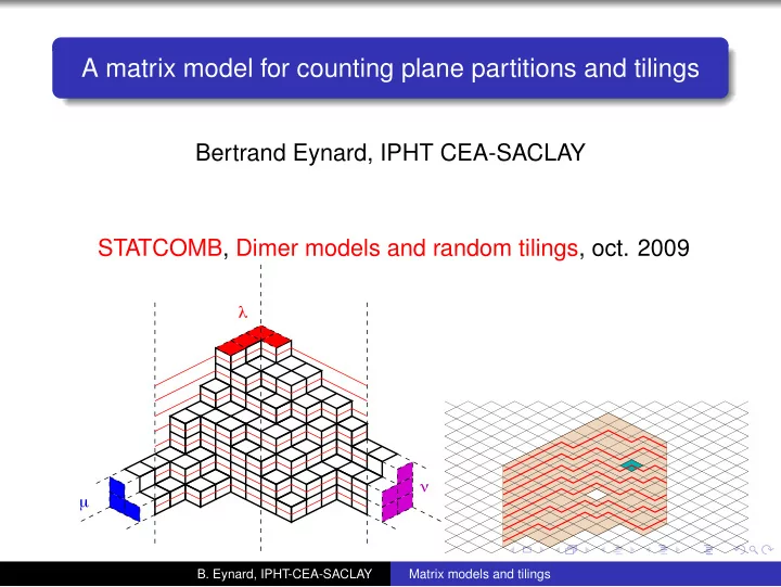
Bertrand Eynard, IPHT CEA-SACLAY STATCOMB, Dimer models and random tilings, oct. 2009
! " µ
- B. Eynard, IPHT-CEA-SACLAY
Matrix models and tilings