A Convolutional Neural Network for Modelling Sentences Nal - - PDF document

Proceedings of the 52nd Annual Meeting of the Association for Computational Linguistics, pages 655–665, Baltimore, Maryland, USA, June 23-25 2014. c 2014 Association for Computational Linguistics

A Convolutional Neural Network for Modelling Sentences

Nal Kalchbrenner Edward Grefenstette

{nal.kalchbrenner, edward.grefenstette, phil.blunsom}@cs.ox.ac.uk

Department of Computer Science University of Oxford Phil Blunsom Abstract

The ability to accurately represent sen- tences is central to language understand-

• ing. We describe a convolutional architec-

ture dubbed the Dynamic Convolutional Neural Network (DCNN) that we adopt for the semantic modelling of sentences. The network uses Dynamic k-Max Pool- ing, a global pooling operation over lin- ear sequences. The network handles input sentences of varying length and induces a feature graph over the sentence that is capable of explicitly capturing short and long-range relations. The network does not rely on a parse tree and is easily ap- plicable to any language. We test the DCNN in four experiments: small scale binary and multi-class sentiment predic- tion, six-way question classification and Twitter sentiment prediction by distant su-

• pervision. The network achieves excellent

performance in the first three tasks and a greater than 25% error reduction in the last task with respect to the strongest baseline.

1 Introduction

The aim of a sentence model is to analyse and represent the semantic content of a sentence for purposes of classification or generation. The sen- tence modelling problem is at the core of many tasks involving a degree of natural language com-

• prehension. These tasks include sentiment analy-

sis, paraphrase detection, entailment recognition, summarisation, discourse analysis, machine trans- lation, grounded language learning and image re-

• trieval. Since individual sentences are rarely ob-

served or not observed at all, one must represent a sentence in terms of features that depend on the words and short n-grams in the sentence that are frequently observed. The core of a sentence model involves a feature function that defines the process

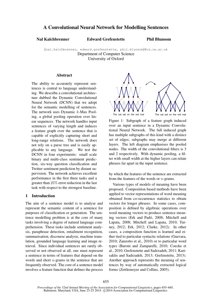
The cat sat on the red mat The cat sat on the red mat

Figure 1: Subgraph of a feature graph induced

• ver an input sentence in a Dynamic Convolu-

tional Neural Network. The full induced graph has multiple subgraphs of this kind with a distinct set of edges; subgraphs may merge at different

• layers. The left diagram emphasises the pooled
• nodes. The width of the convolutional filters is 3

and 2 respectively. With dynamic pooling, a fil- ter with small width at the higher layers can relate phrases far apart in the input sentence. by which the features of the sentence are extracted from the features of the words or n-grams. Various types of models of meaning have been

• proposed. Composition based methods have been

applied to vector representations of word meaning

• btained from co-occurrence statistics to obtain

vectors for longer phrases. In some cases, com- position is defined by algebraic operations over word meaning vectors to produce sentence mean- ing vectors (Erk and Pad´

• , 2008; Mitchell and

Lapata, 2008; Mitchell and Lapata, 2010; Tur- ney, 2012; Erk, 2012; Clarke, 2012). In other cases, a composition function is learned and ei- ther tied to particular syntactic relations (Guevara, 2010; Zanzotto et al., 2010) or to particular word types (Baroni and Zamparelli, 2010; Coecke et al., 2010; Grefenstette and Sadrzadeh, 2011; Kart- saklis and Sadrzadeh, 2013; Grefenstette, 2013). Another approach represents the meaning of sen- tences by way of automatically extracted logical forms (Zettlemoyer and Collins, 2005). 655

A central class of models are those based on neural networks. These range from basic neu- ral bag-of-words or bag-of-n-grams models to the more structured recursive neural networks and to time-delay neural networks based on convo- lutional operations (Collobert and Weston, 2008; Socher et al., 2011; Kalchbrenner and Blunsom, 2013b). Neural sentence models have a num- ber of advantages. They can be trained to obtain generic vectors for words and phrases by predict- ing, for instance, the contexts in which the words and phrases occur. Through supervised training, neural sentence models can fine-tune these vec- tors to information that is specific to a certain

• task. Besides comprising powerful classifiers as

part of their architecture, neural sentence models can be used to condition a neural language model to generate sentences word by word (Schwenk, 2012; Mikolov and Zweig, 2012; Kalchbrenner and Blunsom, 2013a). We define a convolutional neural network archi- tecture and apply it to the semantic modelling of

• sentences. The network handles input sequences
• f varying length. The layers in the network in-

terleave one-dimensional convolutional layers and dynamic k-max pooling layers. Dynamic k-max pooling is a generalisation of the max pooling op-

• erator. The max pooling operator is a non-linear

subsampling function that returns the maximum

• f a set of values (LeCun et al., 1998). The op-

erator is generalised in two respects. First, k- max pooling over a linear sequence of values re- turns the subsequence of k maximum values in the sequence, instead of the single maximum value. Secondly, the pooling parameter k can be dynam- ically chosen by making k a function of other as- pects of the network or the input. The convolutional layers apply

• ne-

dimensional filters across each row of features in the sentence matrix. Convolving the same filter with the n-gram at every position in the sentence allows the features to be extracted independently

• f their position in the sentence. A convolutional

layer followed by a dynamic pooling layer and a non-linearity form a feature map. Like in the convolutional networks for object recognition (LeCun et al., 1998), we enrich the representation in the first layer by computing multiple feature maps with different filters applied to the input sentence. Subsequent layers also have multiple feature maps computed by convolving filters with all the maps from the layer below. The weights at these layers form an order-4 tensor. The resulting architecture is dubbed a Dynamic Convolutional Neural Network. Multiple layers of convolutional and dynamic pooling operations induce a structured feature graph over the input sentence. Figure 1 illustrates such a graph. Small filters at higher layers can cap- ture syntactic or semantic relations between non- continuous phrases that are far apart in the input

• sentence. The feature graph induces a hierarchical

structure somewhat akin to that in a syntactic parse

• tree. The structure is not tied to purely syntactic

relations and is internal to the neural network. We experiment with the network in four set-

• tings. The first two experiments involve predict-

ing the sentiment of movie reviews (Socher et al., 2013b). The network outperforms other ap- proaches in both the binary and the multi-class ex-

• periments. The third experiment involves the cat-

egorisation of questions in six question types in the TREC dataset (Li and Roth, 2002). The net- work matches the accuracy of other state-of-the- art methods that are based on large sets of en- gineered features and hand-coded knowledge re-

• sources. The fourth experiment involves predict-

ing the sentiment of Twitter posts using distant su- pervision (Go et al., 2009). The network is trained

• n 1.6 million tweets labelled automatically ac-

cording to the emoticon that occurs in them. On the hand-labelled test set, the network achieves a greater than 25% reduction in the prediction error with respect to the strongest unigram and bigram baseline reported in Go et al. (2009). The outline of the paper is as follows. Section 2 describes the background to the DCNN including central concepts and related neural sentence mod-

• els. Section 3 defines the relevant operators and

the layers of the network. Section 4 treats of the induced feature graph and other properties of the

• network. Section 5 discusses the experiments and

inspects the learnt feature detectors.1

2 Background

The layers of the DCNN are formed by a convo- lution operation followed by a pooling operation. We begin with a review of related neural sentence

• models. Then we describe the operation of one-

dimensional convolution and the classical Time- Delay Neural Network (TDNN) (Hinton, 1989; Waibel et al., 1990). By adding a max pooling

1Code available at www.nal.co

656

layer to the network, the TDNN can be adopted as a sentence model (Collobert and Weston, 2008). 2.1 Related Neural Sentence Models Various neural sentence models have been de-

• scribed. A general class of basic sentence models

is that of Neural Bag-of-Words (NBoW) models. These generally consist of a projection layer that maps words, sub-word units or n-grams to high dimensional embeddings; the latter are then com- bined component-wise with an operation such as

• summation. The resulting combined vector is clas-

sified through one or more fully connected layers. A model that adopts a more general structure provided by an external parse tree is the Recursive Neural Network (RecNN) (Pollack, 1990; K¨ uchler and Goller, 1996; Socher et al., 2011; Hermann and Blunsom, 2013). At every node in the tree the contexts at the left and right children of the node are combined by a classical layer. The weights of the layer are shared across all nodes in the tree. The layer computed at the top node gives a repre- sentation for the sentence. The Recurrent Neural Network (RNN) is a special case of the recursive network where the structure that is followed is a simple linear chain (Gers and Schmidhuber, 2001; Mikolov et al., 2011). The RNN is primarily used as a language model, but may also be viewed as a sentence model with a linear structure. The layer computed at the last word represents the sentence. Finally, a further class of neural sentence mod- els is based on the convolution operation and the TDNN architecture (Collobert and Weston, 2008; Kalchbrenner and Blunsom, 2013b). Certain con- cepts used in these models are central to the DCNN and we describe them next. 2.2 Convolution The one-dimensional convolution is an operation between a vector of weights m ∈ Rm and a vector

• f inputs viewed as a sequence s ∈ Rs. The vector

m is the filter of the convolution. Concretely, we think of s as the input sentence and si ∈ R is a sin- gle feature value associated with the i-th word in the sentence. The idea behind the one-dimensional convolution is to take the dot product of the vector m with each m-gram in the sentence s to obtain another sequence c: cj = m⊺sj−m+1:j (1) Equation 1 gives rise to two types of convolution depending on the range of the index j. The narrow type of convolution requires that s ≥ m and yields

s1 s1 ss ss c1 c5 c5

Figure 2: Narrow and wide types of convolution. The filter m has size m = 5. a sequence c ∈ Rs−m+1 with j ranging from m to s. The wide type of convolution does not have requirements on s or m and yields a sequence c ∈ Rs+m−1 where the index j ranges from 1 to s + m − 1. Out-of-range input values si where i < 1

• r i > s are taken to be zero. The result of the

narrow convolution is a subsequence of the result

• f the wide convolution. The two types of one-

dimensional convolution are illustrated in Fig. 2. The trained weights in the filter m correspond to a linguistic feature detector that learns to recog- nise a specific class of n-grams. These n-grams have size n ≤ m, where m is the width of the

• filter. Applying the weights m in a wide convo-

lution has some advantages over applying them in a narrow one. A wide convolution ensures that all weights in the filter reach the entire sentence, in- cluding the words at the margins. This is particu- larly significant when m is set to a relatively large value such as 8 or 10. In addition, a wide convo- lution guarantees that the application of the filter m to the input sentence s always produces a valid non-empty result c, independently of the width m and the sentence length s. We next describe the classical convolutional layer of a TDNN. 2.3 Time-Delay Neural Networks A TDNN convolves a sequence of inputs s with a set of weights m. As in the TDNN for phoneme recognition (Waibel et al., 1990), the sequence s is viewed as having a time dimension and the con- volution is applied over the time dimension. Each sj is often not just a single value, but a vector of d values so that s ∈ Rd×s. Likewise, m is a ma- trix of weights of size d × m. Each row of m is convolved with the corresponding row of s and the convolution is usually of the narrow type. Multi- ple convolutional layers may be stacked by taking the resulting sequence c as input to the next layer. The Max-TDNN sentence model is based on the architecture of a TDNN (Collobert and Weston, 2008). In the model, a convolutional layer of the narrow type is applied to the sentence matrix s, where each column corresponds to the feature vec- 657

tor wi ∈ Rd of a word in the sentence: s =  w1 . . . ws   (2) To address the problem of varying sentence lengths, the Max-TDNN takes the maximum of each row in the resulting matrix c yielding a vector

• f d values:

cmax =    max(c1,:) . . . max(cd,:)    (3) The aim is to capture the most relevant feature, i.e. the one with the highest value, for each of the d rows of the resulting matrix c. The fixed-sized vector cmax is then used as input to a fully con- nected layer for classification. The Max-TDNN model has many desirable

• properties. It is sensitive to the order of the words

in the sentence and it does not depend on external language-specific features such as dependency or constituency parse trees. It also gives largely uni- form importance to the signal coming from each

• f the words in the sentence, with the exception
• f words at the margins that are considered fewer

times in the computation of the narrow convolu-

• tion. But the model also has some limiting as-
• pects. The range of the feature detectors is lim-

ited to the span m of the weights. Increasing m or stacking multiple convolutional layers of the nar- row type makes the range of the feature detectors larger; at the same time it also exacerbates the ne- glect of the margins of the sentence and increases the minimum size s of the input sentence required by the convolution. For this reason higher-order and long-range feature detectors cannot be easily incorporated into the model. The max pooling op- eration has some disadvantages too. It cannot dis- tinguish whether a relevant feature in one of the rows occurs just one or multiple times and it for- gets the order in which the features occur. More generally, the pooling factor by which the signal

• f the matrix is reduced at once corresponds to

s−m+1; even for moderate values of s the pool- ing factor can be excessive. The aim of the next section is to address these limitations while pre- serving the advantages.

3 Convolutional Neural Networks with Dynamic k-Max Pooling

We model sentences using a convolutional archi- tecture that alternates wide convolutional layers

K-Max pooling (k=3) Fully connected layer Folding Wide convolution (m=2) Dynamic k-max pooling (k= f(s) =5) Projected sentence matrix (s=7) Wide convolution (m=3) The cat sat on the red mat

Figure 3: A DCNN for the seven word input sen-

• tence. Word embeddings have size d = 4. The

network has two convolutional layers with two feature maps each. The widths of the filters at the two layers are respectively 3 and 2. The (dynamic) k-max pooling layers have values k of 5 and 3. with dynamic pooling layers given by dynamic k- max pooling. In the network the width of a feature map at an intermediate layer varies depending on the length of the input sentence; the resulting ar- chitecture is the Dynamic Convolutional Neural

• Network. Figure 3 represents a DCNN. We pro-

ceed to describe the network in detail. 3.1 Wide Convolution Given an input sentence, to obtain the first layer of the DCNN we take the embedding wi ∈ Rd for each word in the sentence and construct the sen- tence matrix s ∈ Rd×s as in Eq. 2. The values in the embeddings wi are parameters that are op- timised during training. A convolutional layer in the network is obtained by convolving a matrix of weights m ∈ Rd×m with the matrix of activations at the layer below. For example, the second layer is obtained by applying a convolution to the sen- tence matrix s itself. Dimension d and filter width m are hyper-parameters of the network. We let the

• perations be wide one-dimensional convolutions

as described in Sect. 2.2. The resulting matrix c has dimensions d × (s + m − 1). 658

3.2 k-Max Pooling We next describe a pooling operation that is a gen- eralisation of the max pooling over the time di- mension used in the Max-TDNN sentence model and different from the local max pooling opera- tions applied in a convolutional network for object recognition (LeCun et al., 1998). Given a value k and a sequence p ∈ Rp of length p ≥ k, k- max pooling selects the subsequence pk

max of the

k highest values of p. The order of the values in pk

max corresponds to their original order in p.

The k-max pooling operation makes it possible to pool the k most active features in p that may be a number of positions apart; it preserves the order

• f the features, but is insensitive to their specific
• positions. It can also discern more finely the num-

ber of times the feature is highly activated in p and the progression by which the high activations

• f the feature change across p. The k-max pooling
• perator is applied in the network after the topmost

convolutional layer. This guarantees that the input to the fully connected layers is independent of the length of the input sentence. But, as we see next, at intermediate convolutional layers the pooling pa- rameter k is not fixed, but is dynamically selected in order to allow for a smooth extraction of higher-

• rder and longer-range features.

3.3 Dynamic k-Max Pooling A dynamic k-max pooling operation is a k-max pooling operation where we let k be a function of the length of the sentence and the depth of the net-

• work. Although many functions are possible, we

simply model the pooling parameter as follows: kl = max( ktop, ⌈L − l L s⌉ ) (4) where l is the number of the current convolutional layer to which the pooling is applied and L is the total number of convolutional layers in the net- work; ktop is the fixed pooling parameter for the topmost convolutional layer (Sect. 3.2). For in- stance, in a network with three convolutional lay- ers and ktop = 3, for an input sentence of length s = 18, the pooling parameter at the first layer is k1 = 12 and the pooling parameter at the sec-

• nd layer is k2 = 6; the third layer has the fixed

pooling parameter k3 = ktop = 3. Equation 4 is a model of the number of values needed to de- scribe the relevant parts of the progression of an l-th order feature over a sentence of length s. For an example in sentiment prediction, according to the equation a first order feature such as a posi- tive word occurs at most k1 times in a sentence of length s, whereas a second order feature such as a negated phrase or clause occurs at most k2 times. 3.4 Non-linear Feature Function After (dynamic) k-max pooling is applied to the result of a convolution, a bias b ∈ Rd and a non- linear function g are applied component-wise to the pooled matrix. There is a single bias value for each row of the pooled matrix. If we temporarily ignore the pooling layer, we may state how one computes each d-dimensional column a in the matrix a resulting after the convo- lutional and non-linear layers. Define M to be the matrix of diagonals: M = [diag(m:,1), . . . , diag(m:,m)] (5) where m are the weights of the d filters of the wide

• convolution. Then after the first pair of a convolu-

tional and a non-linear layer, each column a in the matrix a is obtained as follows, for some index j: a = g   M    wj . . . wj+m−1    + b    (6) Here a is a column of first order features. Sec-

• nd order features are similarly obtained by ap-

plying Eq. 6 to a sequence of first order features aj, ..., aj+m′−1 with another weight matrix M′. Barring pooling, Eq. 6 represents a core aspect

• f the feature extraction function and has a rather

general form that we return to below. Together with pooling, the feature function induces position invariance and makes the range of higher-order features variable. 3.5 Multiple Feature Maps So far we have described how one applies a wide convolution, a (dynamic) k-max pooling layer and a non-linear function to the input sentence ma- trix to obtain a first order feature map. The three

• perations can be repeated to yield feature maps
• f increasing order and a network of increasing
• depth. We denote a feature map of the i-th order

by Fi. As in convolutional networks for object recognition, to increase the number of learnt fea- ture detectors of a certain order, multiple feature maps Fi

1, . . . , Fi n may be computed in parallel at

the same layer. Each feature map Fi

j is computed

by convolving a distinct set of filters arranged in a matrix mi

j,k with each feature map Fi−1 k

• f the

lower order i − 1 and summing the results: 659

Fi

j = n

• k=1

mi

j,k ∗ Fi−1 k

(7) where ∗ indicates the wide convolution. The weights mi

j,k form an order-4 tensor. After the

wide convolution, first dynamic k-max pooling and then the non-linear function are applied indi- vidually to each map. 3.6 Folding In the formulation of the network so far, feature detectors applied to an individual row of the sen- tence matrix s can have many orders and create complex dependencies across the same rows in multiple feature maps. Feature detectors in differ- ent rows, however, are independent of each other until the top fully connected layer. Full depen- dence between different rows could be achieved by making M in Eq. 5 a full matrix instead of a sparse matrix of diagonals. Here we explore a simpler method called folding that does not intro- duce any additional parameters. After a convo- lutional layer and before (dynamic) k-max pool- ing, one just sums every two rows in a feature map component-wise. For a map of d rows, folding re- turns a map of d/2 rows, thus halving the size of the representation. With a folding layer, a feature detector of the i-th order depends now on two rows

• f feature values in the lower maps of order i − 1.

This ends the description of the DCNN.

4 Properties of the Sentence Model

We describe some of the properties of the sentence model based on the DCNN. We describe the no- tion of the feature graph induced over a sentence by the succession of convolutional and pooling

• layers. We briefly relate the properties to those of
• ther neural sentence models.

4.1 Word and n-Gram Order One of the basic properties is sensitivity to the or- der of the words in the input sentence. For most applications and in order to learn fine-grained fea- ture detectors, it is beneficial for a model to be able to discriminate whether a specific n-gram occurs in the input. Likewise, it is beneficial for a model to be able to tell the relative position of the most relevant n-grams. The network is designed to cap- ture these two aspects. The filters m of the wide convolution in the first layer can learn to recognise specific n-grams that have size less or equal to the filter width m; as we see in the experiments, m in the first layer is often set to a relatively large value such as 10. The subsequence of n-grams extracted by the generalised pooling operation induces in- variance to absolute positions, but maintains their

• rder and relative positions.

As regards the other neural sentence models, the class of NBoW models is by definition insensitive to word order. A sentence model based on a recur- rent neural network is sensitive to word order, but it has a bias towards the latest words that it takes as input (Mikolov et al., 2011). This gives the RNN excellent performance at language modelling, but it is suboptimal for remembering at once the n- grams further back in the input sentence. Sim- ilarly, a recursive neural network is sensitive to word order but has a bias towards the topmost nodes in the tree; shallower trees mitigate this ef- fect to some extent (Socher et al., 2013a). As seen in Sect. 2.3, the Max-TDNN is sensitive to word

• rder, but max pooling only picks out a single n-

gram feature in each row of the sentence matrix. 4.2 Induced Feature Graph Some sentence models use internal or external structure to compute the representation for the in- put sentence. In a DCNN, the convolution and pooling layers induce an internal feature graph

• ver the input. A node from a layer is connected

to a node from the next higher layer if the lower node is involved in the convolution that computes the value of the higher node. Nodes that are not selected by the pooling operation at a layer are dropped from the graph. After the last pooling layer, the remaining nodes connect to a single top- most root. The induced graph is a connected, di- rected acyclic graph with weighted edges and a root node; two equivalent representations of an induced graph are given in Fig. 1. In a DCNN without folding layers, each of the d rows of the sentence matrix induces a subgraph that joins the

• ther subgraphs only at the root node. Each sub-

graph may have a different shape that reflects the kind of relations that are detected in that subgraph. The effect of folding layers is to join pairs of sub- graphs at lower layers before the top root node. Convolutional networks for object recognition also induce a feature graph over the input image. What makes the feature graph of a DCNN pecu- liar is the global range of the pooling operations. The (dynamic) k-max pooling operator can draw together features that correspond to words that are many positions apart in the sentence. Higher-order features have highly variable ranges that can be ei- 660

ther short and focused or global and long as the input sentence. Likewise, the edges of a subgraph in the induced graph reflect these varying ranges. The subgraphs can either be localised to one or more parts of the sentence or spread more widely across the sentence. This structure is internal to the network and is defined by the forward propa- gation of the input through the network. Of the other sentence models, the NBoW is a shallow model and the RNN has a linear chain structure. The subgraphs induced in the Max- TDNN model have a single fixed-range feature ob- tained through max pooling. The recursive neural network follows the structure of an external parse

• tree. Features of variable range are computed at

each node of the tree combining one or more of the children of the tree. Unlike in a DCNN, where

• ne learns a clear hierarchy of feature orders, in

a RecNN low order features like those of sin- gle words can be directly combined with higher

• rder features computed from entire clauses. A

DCNN generalises many of the structural aspects

• f a RecNN. The feature extraction function as

stated in Eq. 6 has a more general form than that in a RecNN, where the value of m is generally 2. Likewise, the induced graph structure in a DCNN is more general than a parse tree in that it is not limited to syntactically dictated phrases; the graph structure can capture short or long-range seman- tic relations between words that do not necessar- ily correspond to the syntactic relations in a parse tree. The DCNN has internal input-dependent structure and does not rely on externally provided parse trees, which makes the DCNN directly ap- plicable to hard-to-parse sentences such as tweets and to sentences from any language.

5 Experiments

We test the network on four different experiments. We begin by specifying aspects of the implemen- tation and the training of the network. We then re- late the results of the experiments and we inspect the learnt feature detectors. 5.1 Training In each of the experiments, the top layer of the network has a fully connected layer followed by a softmax non-linearity that predicts the probabil- ity distribution over classes given the input sen- tence. The network is trained to minimise the cross-entropy of the predicted and true distribu- tions; the objective includes an L2 regularisation

Classifier Fine-grained (%) Binary (%) NB 41.0 81.8 BINB 41.9 83.1 SVM 40.7 79.4 RECNTN 45.7 85.4 MAX-TDNN 37.4 77.1 NBOW 42.4 80.5 DCNN 48.5 86.8

Table 1: Accuracy of sentiment prediction in the movie reviews dataset. The first four results are reported from Socher et al. (2013b). The baselines NB and BINB are Naive Bayes classifiers with, respectively, unigram features and unigram and bi- gram features. SVM is a support vector machine with unigram and bigram features. RECNTN is a recursive neural network with a tensor-based fea- ture function, which relies on external structural features given by a parse tree and performs best among the RecNNs. term over the parameters. The set of parameters comprises the word embeddings, the filter weights and the weights from the fully connected layers. The network is trained with mini-batches by back- propagation and the gradient-based optimisation is performed using the Adagrad update rule (Duchi et al., 2011). Using the well-known convolution theorem, we can compute fast one-dimensional linear convolutions at all rows of an input matrix by using Fast Fourier Transforms. To exploit the parallelism of the operations, we train the network

• n a GPU. A Matlab implementation processes

multiple millions of input sentences per hour on

• ne GPU, depending primarily on the number of

layers used in the network. 5.2 Sentiment Prediction in Movie Reviews The first two experiments concern the prediction

• f the sentiment of movie reviews in the Stanford

Sentiment Treebank (Socher et al., 2013b). The

• utput variable is binary in one experiment and

can have five possible outcomes in the other: neg- ative, somewhat negative, neutral, somewhat posi- tive, positive. In the binary case, we use the given splits of 6920 training, 872 development and 1821 test sentences. Likewise, in the fine-grained case, we use the standard 8544/1101/2210 splits. La- belled phrases that occur as subparts of the train- ing sentences are treated as independent training

• instances. The size of the vocabulary is 15448.

Table 1 details the results of the experiments. 661

Classifier Features

• Acc. (%)

HIER unigram, POS, head chunks 91.0 NE, semantic relations MAXENT unigram, bigram, trigram 92.6 POS, chunks, NE, supertags CCG parser, WordNet MAXENT unigram, bigram, trigram 93.6 POS, wh-word, head word word shape, parser hypernyms, WordNet SVM unigram, POS, wh-word 95.0 head word, parser hypernyms, WordNet 60 hand-coded rules MAX-TDNN unsupervised vectors 84.4 NBOW unsupervised vectors 88.2 DCNN unsupervised vectors 93.0

Table 2: Accuracy of six-way question classifica- tion on the TREC questions dataset. The second column details the external features used in the various approaches. The first four results are re- spectively from Li and Roth (2002), Blunsom et al. (2006), Huang et al. (2008) and Silva et al. (2011). In the three neural sentence models—the Max- TDNN, the NBoW and the DCNN—the word vec- tors are parameters of the models that are ran- domly initialised; their dimension d is set to 48. The Max-TDNN has a filter of width 6 in its nar- row convolution at the first layer; shorter phrases are padded with zero vectors. The convolu- tional layer is followed by a non-linearity, a max- pooling layer and a softmax classification layer. The NBoW sums the word vectors and applies a non-linearity followed by a softmax classification

• layer. The adopted non-linearity is the tanh func-
• tion. The hyper parameters of the DCNN are as
• follows. The binary result is based on a DCNN

that has a wide convolutional layer followed by a folding layer, a dynamic k-max pooling layer and a non-linearity; it has a second wide convolutional layer followed by a folding layer, a k-max pooling layer and a non-linearity. The width of the convo- lutional filters is 7 and 5, respectively. The value

• f k for the top k-max pooling is 4. The num-

ber of feature maps at the first convolutional layer is 6; the number of maps at the second convolu- tional layer is 14. The network is topped by a soft- max classification layer. The DCNN for the fine- grained result has the same architecture, but the filters have size 10 and 7, the top pooling parame- ter k is 5 and the number of maps is, respectively, 6 and 12. The networks use the tanh non-linear

Classifier Accuracy (%) SVM 81.6 BINB 82.7 MAXENT 83.0 MAX-TDNN 78.8 NBOW 80.9 DCNN 87.4

Table 3: Accuracy on the Twitter sentiment

• dataset. The three non-neural classifiers are based
• n unigram and bigram features; the results are re-

ported from (Go et al., 2009).

• function. At training time we apply dropout to the

penultimate layer after the last tanh non-linearity (Hinton et al., 2012). We see that the DCNN significantly outper- forms the other neural and non-neural models. The NBoW performs similarly to the non-neural n-gram based classifiers. The Max-TDNN per- forms worse than the NBoW likely due to the ex- cessive pooling of the max pooling operation; the latter discards most of the sentiment features of the words in the input sentence. Besides the RecNN that uses an external parser to produce structural features for the model, the other models use n- gram based or neural features that do not require external resources or additional annotations. In the next experiment we compare the performance of the DCNN with those of methods that use heavily engineered resources. 5.3 Question Type Classification As an aid to question answering, a question may be classified as belonging to one of many question

• types. The TREC questions dataset involves six

different question types, e.g. whether the question is about a location, about a person or about some numeric information (Li and Roth, 2002). The training dataset consists of 5452 labelled questions whereas the test dataset consists of 500 questions. The results are reported in Tab. 2. The non- neural approaches use a classifier over a large number of manually engineered features and hand-coded resources. For instance, Blunsom et

• al. (2006) present a Maximum Entropy model that

relies on 26 sets of syntactic and semantic fea- tures including unigrams, bigrams, trigrams, POS tags, named entity tags, structural relations from a CCG parse and WordNet synsets. We evaluate the three neural models on this dataset with mostly the same hyper-parameters as in the binary senti- 662

POSITIVE lovely ! ! ! ! !comedic ! ! ! ! !moments !and ! ! ! !several ! ! ! ! !fine ! ! ! ! ! !performances good ! ! ! ! ! ! !script ! ! ! ! ! !, ! ! ! ! ! ! !good ! ! !dialogue ! ! ! !, ! ! ! ! ! ! ! ! !funny ! ! ! ! ! ! ! sustains ! ! !throughout ! !is ! ! ! ! ! !daring !, ! ! ! ! ! ! ! ! ! ! !inventive !and ! ! ! ! ! ! ! ! ! well ! ! ! ! ! ! !written ! ! ! ! !, ! ! ! ! ! ! !nicely !acted ! ! ! ! ! ! !and ! ! ! ! ! ! !beautifully ! remarkably !solid ! ! ! ! ! ! !and ! ! ! ! !subtly !satirical ! ! !tour ! ! ! ! ! !de ! ! ! ! ! ! ! ! ! ! NEGATIVE , ! ! ! ! ! ! ! ! ! !nonexistent !plot ! ! ! !and ! ! ! !pretentious !visual ! ! ! !style ! ! ! ! ! ! ! it ! ! ! ! ! ! ! ! !fails ! ! ! ! ! ! !the ! ! ! ! !most ! ! !basic ! ! ! ! ! ! !test ! ! ! ! ! !as ! ! ! ! ! ! ! ! ! ! so ! ! ! ! ! ! ! ! !stupid ! ! ! ! ! !, ! ! ! ! ! ! !so ! ! ! ! !ill ! ! ! ! ! ! ! ! !conceived !, ! ! ! ! ! ! ! ! ! ! ! , ! ! ! ! ! ! ! ! ! !too ! ! ! ! ! ! ! ! !dull ! ! ! !and ! ! ! !pretentious !to ! ! ! ! ! ! ! !be ! ! ! ! ! ! ! ! ! ! hood ! ! ! ! ! ! !rats ! ! ! ! ! ! ! !butt ! ! ! !their ! !ugly ! ! ! ! ! ! ! !heads ! ! ! ! !in ! ! ! ! ! ! ! ! ! ! ! ! ! ! ! ! ! ! ! 'NOT' n't ! ! ! !have ! ! ! ! !any ! ! ! ! ! ! ! ! !huge !laughs ! ! ! ! ! !in ! ! ! ! ! ! ! ! ! ! !its ! ! ! no ! ! ! ! !movement !, ! ! ! ! ! ! ! ! ! ! !no ! ! !, ! ! ! ! ! ! ! ! ! ! !not ! ! ! ! ! ! ! ! ! !much ! ! n't ! ! ! !stop ! ! ! ! !me ! ! ! ! ! ! ! ! ! !from !enjoying ! ! ! !much ! ! ! ! ! ! ! ! !of ! ! ! ! not ! ! ! !that ! ! ! ! !kung ! ! ! ! ! ! ! !pow ! !is ! ! ! ! ! ! ! ! ! !n't ! ! ! ! ! ! ! ! ! !funny ! not ! ! ! !a ! ! ! ! ! ! ! !moment ! ! ! ! ! !that !is ! ! ! ! ! ! ! ! ! !not ! ! ! ! ! ! ! ! ! !false ! 'TOO' , ! ! ! ! ! !too ! ! ! ! ! !dull ! ! ! ! ! ! ! !and ! !pretentious !to ! ! ! ! ! ! ! ! ! ! !be ! ! ! ! ! ! ! ! either !too ! ! ! ! ! !serious ! ! ! ! !or ! ! !too ! ! ! ! ! ! ! ! !lighthearted !, ! ! ! ! ! ! ! ! ! too ! ! ! !slow ! ! ! ! !, ! ! ! ! ! ! ! ! ! ! !too ! !long ! ! ! ! ! ! ! !and ! ! ! ! ! ! ! ! ! !too ! ! ! ! ! ! ! feels ! !too ! ! ! ! ! !formulaic ! ! !and ! !too ! ! ! ! ! ! ! ! !familiar ! ! ! ! !to ! ! ! ! ! ! ! ! is ! ! ! ! !too ! ! ! ! ! !predictable !and ! !too ! ! ! ! ! ! ! ! !self ! ! ! ! ! ! ! ! !conscious ! !

Figure 4: Top five 7-grams at four feature detectors in the first layer of the network. ment experiment of Sect. 5.2. As the dataset is rather small, we use lower-dimensional word vec- tors with d = 32 that are initialised with embed- dings trained in an unsupervised way to predict contexts of occurrence (Turian et al., 2010). The DCNN uses a single convolutional layer with fil- ters of size 8 and 5 feature maps. The difference between the performance of the DCNN and that of the other high-performing methods in Tab. 2 is not significant (p < 0.09). Given that the only labelled information used to train the network is the train- ing set itself, it is notable that the network matches the performance of state-of-the-art classifiers that rely on large amounts of engineered features and rules and hand-coded resources. 5.4 Twitter Sentiment Prediction with Distant Supervision In our final experiment, we train the models on a large dataset of tweets, where a tweet is automat- ically labelled as positive or negative depending

• n the emoticon that occurs in it. The training set

consists of 1.6 million tweets with emoticon-based labels and the test set of about 400 hand-annotated

• tweets. We preprocess the tweets minimally fol-

lowing the procedure described in Go et al. (2009); in addition, we also lowercase all the tokens. This results in a vocabulary of 76643 word types. The architecture of the DCNN and of the other neural models is the same as the one used in the binary experiment of Sect. 5.2. The randomly initialised word embeddings are increased in length to a di- mension of d = 60. Table 3 reports the results of the experiments. We see a significant increase in the performance of the DCNN with respect to the non-neural n-gram based classifiers; in the pres- ence of large amounts of training data these clas- sifiers constitute particularly strong baselines. We see that the ability to train a sentiment classifier on automatically extracted emoticon-based labels ex- tends to the DCNN and results in highly accurate

• performance. The difference in performance be-

tween the DCNN and the NBoW further suggests that the ability of the DCNN to both capture fea- tures based on long n-grams and to hierarchically combine these features is highly beneficial. 5.5 Visualising Feature Detectors A filter in the DCNN is associated with a feature detector or neuron that learns during training to be particularly active when presented with a spe- cific sequence of input words. In the first layer, the sequence is a continuous n-gram from the input sentence; in higher layers, sequences can be made

• f multiple separate n-grams.

We visualise the feature detectors in the first layer of the network trained on the binary sentiment task (Sect. 5.2). Since the filters have width 7, for each of the 288 feature detectors we rank all 7-grams occurring in the validation and test sets according to their ac- tivation of the detector. Figure 5.2 presents the top five 7-grams for four feature detectors. Be- sides the expected detectors for positive and nega- tive sentiment, we find detectors for particles such as ‘not’ that negate sentiment and such as ‘too’ that potentiate sentiment. We find detectors for multiple other notable constructs including ‘all’, ‘or’, ‘with...that’, ‘as...as’. The feature detectors learn to recognise not just single n-grams, but pat- terns within n-grams that have syntactic, semantic

• r structural significance.

6 Conclusion

We have described a dynamic convolutional neural network that uses the dynamic k-max pooling op- erator as a non-linear subsampling function. The feature graph induced by the network is able to capture word relations of varying size. The net- work achieves high performance on question and sentiment classification without requiring external features as provided by parsers or other resources.

Acknowledgements

We thank Nando de Freitas and Yee Whye Teh for great discussions on the paper. This work was supported by a Xerox Foundation Award, EPSRC grant number EP/F042728/1, and EPSRC grant number EP/K036580/1. 663

References

Marco Baroni and Roberto Zamparelli. 2010. Nouns are vectors, adjectives are matrices: Representing adjective-noun constructions in semantic space. In EMNLP, pages 1183–1193. ACL. Phil Blunsom, Krystle Kocik, and James R. Curran.

• 2006. Question classification with log-linear mod-

els. In SIGIR ’06: Proceedings of the 29th an- nual international ACM SIGIR conference on Re- search and development in information retrieval, pages 615–616, New York, NY, USA. ACM. Daoud Clarke. 2012. A context-theoretic frame- work for compositionality in distributional seman-

• tics. Computational Linguistics, 38(1):41–71.

Bob Coecke, Mehrnoosh Sadrzadeh, and Stephen

• Clark. 2010. Mathematical Foundations for a Com-

positional Distributional Model of Meaning. March. Ronan Collobert and Jason Weston. 2008. A unified architecture for natural language processing: Deep neural networks with multitask learning. In Interna- tional Conference on Machine Learning, ICML. John Duchi, Elad Hazan, and Yoram Singer. 2011. Adaptive subgradient methods for online learning and stochastic optimization. J. Mach. Learn. Res., 12:2121–2159, July. Katrin Erk and Sebastian Pad´

• . 2008. A structured

vector space model for word meaning in context. Proceedings of the Conference on Empirical Meth-

• ds in Natural Language Processing - EMNLP ’08,

(October):897. Katrin Erk. 2012. Vector space models of word mean- ing and phrase meaning: A survey. Language and Linguistics Compass, 6(10):635–653. Felix A. Gers and Jrgen Schmidhuber. 2001. Lstm recurrent networks learn simple context-free and context-sensitive languages. IEEE Transactions on Neural Networks, 12(6):1333–1340. Alec Go, Richa Bhayani, and Lei Huang. 2009. Twit- ter sentiment classification using distant supervision. Processing, pages 1–6. Edward Grefenstette and Mehrnoosh Sadrzadeh. 2011. Experimental support for a categorical composi- tional distributional model of meaning. In Proceed- ings of the Conference on Empirical Methods in Nat- ural Language Processing, pages 1394–1404. Asso- ciation for Computational Linguistics. Edward Grefenstette. 2013. Category-theoretic quantitative compositional distributional models

• f natural language semantics.

arXiv preprint arXiv:1311.1539. Emiliano Guevara. 2010. Modelling Adjective-Noun Compositionality by Regression. ESSLLI’10 Work- shop on Compositionality and Distributional Se- mantic Models. Karl Moritz Hermann and Phil Blunsom. 2013. The Role of Syntax in Vector Space Models of Composi- tional Semantics. In Proceedings of the 51st Annual Meeting of the Association for Computational Lin- guistics (Volume 1: Long Papers), Sofia, Bulgaria,

• August. Association for Computational Linguistics.

Forthcoming. Geoffrey E. Hinton, Nitish Srivastava, Alex Krizhevsky, Ilya Sutskever, and Ruslan Salakhut- dinov. 2012. Improving neural networks by preventing co-adaptation

• f

feature detectors. CoRR, abs/1207.0580. Geoffrey E. Hinton. 1989. Connectionist learning pro-

• cedures. Artif. Intell., 40(1-3):185–234.

Zhiheng Huang, Marcus Thint, and Zengchang Qin.

• 2008. Question classification using head words and

their hypernyms. In Proceedings of the Conference

• n Empirical Methods in Natural Language Pro-

cessing, EMNLP ’08, pages 927–936, Stroudsburg, PA, USA. Association for Computational Linguis- tics. Nal Kalchbrenner and Phil Blunsom. 2013a. Recur- rent continuous translation models. In Proceedings

• f the 2013 Conference on Empirical Methods in

Natural Language Processing, Seattle, October. As- sociation for Computational Linguistics. Nal Kalchbrenner and Phil Blunsom. 2013b. Recur- rent Convolutional Neural Networks for Discourse

• Compositionality. In Proceedings of the Workshop
• n Continuous Vector Space Models and their Com-

positionality, Sofia, Bulgaria, August. Association for Computational Linguistics. Dimitri Kartsaklis and Mehrnoosh Sadrzadeh. 2013. Prior disambiguation of word tensors for construct- ing sentence vectors. In Proceedings of the 2013 Conference on Empirical Methods in Natural Lan- guage Processing (EMNLP), Seattle, USA, October. Andreas K¨ uchler and Christoph Goller. 1996. Induc- tive learning in symbolic domains using structure- driven recurrent neural networks. In G¨ unther G¨

• rz

and Steffen H¨

• lldobler, editors, KI, volume 1137 of

Lecture Notes in Computer Science, pages 183–197. Springer. Yann LeCun, L´ eon Bottou, Yoshua Bengio, and Patrick

• Haffner. 1998. Gradient-based learning applied to

document recognition. Proceedings of the IEEE, 86(11):2278–2324, November. Xin Li and Dan Roth. 2002. Learning question clas- sifiers. In Proceedings of the 19th international conference on Computational linguistics-Volume 1, pages 1–7. Association for Computational Linguis- tics. Tomas Mikolov and Geoffrey Zweig. 2012. Context dependent recurrent neural network language model. In SLT, pages 234–239.

664

Tomas Mikolov, Stefan Kombrink, Lukas Burget, Jan Cernock´ y, and Sanjeev Khudanpur. 2011. Exten- sions of recurrent neural network language model. In ICASSP, pages 5528–5531. IEEE. Jeff Mitchell and Mirella Lapata. 2008. Vector-based models of semantic composition. In Proceedings of ACL, volume 8. Jeff Mitchell and Mirella Lapata. 2010. Composition in distributional models of semantics. Cognitive Sci- ence, 34(8):1388–1429. Jordan B. Pollack. 1990. Recursive distributed repre-

• sentations. Artificial Intelligence, 46:77–105.

Holger Schwenk. 2012. Continuous space translation models for phrase-based statistical machine transla-

• tion. In COLING (Posters), pages 1071–1080.

Joo Silva, Lusa Coheur, AnaCristina Mendes, and An- dreas Wichert. 2011. From symbolic to sub- symbolic information in question classification. Ar- tificial Intelligence Review, 35(2):137–154. Richard Socher, Jeffrey Pennington, Eric H. Huang, Andrew Y. Ng, and Christopher D. Manning. 2011. Semi-Supervised Recursive Autoencoders for Pre- dicting Sentiment Distributions. In Proceedings of the 2011 Conference on Empirical Methods in Nat- ural Language Processing (EMNLP). Richard Socher, Quoc V. Le, Christopher D. Manning, and Andrew Y. Ng. 2013a. Grounded Composi- tional Semantics for Finding and Describing Images with Sentences. In Transactions of the Association for Computational Linguistics (TACL). Richard Socher, Alex Perelygin, Jean Wu, Jason Chuang, Christopher D. Manning, Andrew Y. Ng, and Christopher Potts. 2013b. Recursive deep mod- els for semantic compositionality over a sentiment

• treebank. In Proceedings of the 2013 Conference on

Empirical Methods in Natural Language Process- ing, pages 1631–1642, Stroudsburg, PA, October. Association for Computational Linguistics. Joseph Turian, Lev Ratinov, and Yoshua Bengio. 2010. Word representations: a simple and general method for semi-supervised learning. In Proceedings of the 48th Annual Meeting of the Association for Compu- tational Linguistics, pages 384–394. Association for Computational Linguistics. Peter Turney. 2012. Domain and function: A dual- space model of semantic relations and compositions.

• J. Artif. Intell. Res.(JAIR), 44:533–585.

Alexander Waibel, Toshiyuki Hanazawa, Geofrey Hin- ton, Kiyohiro Shikano, and Kevin J. Lang. 1990. Readings in speech recognition. chapter Phoneme Recognition Using Time-delay Neural Networks, pages 393–404. Morgan Kaufmann Publishers Inc., San Francisco, CA, USA. Fabio Massimo Zanzotto, Ioannis Korkontzelos, Francesca Fallucchi, and Suresh Manandhar. 2010. Estimating linear models for compositional distri- butional semantics. In Proceedings of the 23rd In- ternational Conference on Computational Linguis- tics, pages 1263–1271. Association for Computa- tional Linguistics. Luke S. Zettlemoyer and Michael Collins. 2005. Learning to map sentences to logical form: Struc- tured classification with probabilistic categorial

• grammars. In UAI, pages 658–666. AUAI Press.

665