
SLIDE 1
A Carbuncle-free Roe-Type Solver for the Euler Equations
Friedemann Kemm BTU Cottbus kemm@math.tu-cottbus.de
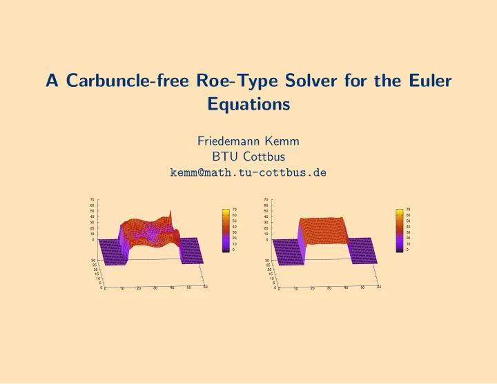
10 20 30 40 50 60 70 10 20 30 40 50 60 5 10 15 20 25 30 10 20 30 40 50 60 70 10 20 30 40 50 60 70 10 20 30 40 50 60 5 10 15 20 25 30 10 20 30 40 50 60 70