6. (3 pts) What three things form the deadly triad the three - - PowerPoint PPT Presentation

6 3 pts what three things form the deadly triad the three
SMART_READER_LITE
LIVE PREVIEW

6. (3 pts) What three things form the deadly triad the three - - PowerPoint PPT Presentation

6. (3 pts) What three things form the deadly triad the three things that cannot be combined in the same learning situation without risking divergence? (circle three) (a) eligibility traces (b) bootstrapping (c) sample backups (d)


slide-1
SLIDE 1
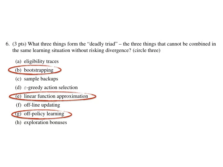
  • 6. (3 pts) What three things form the “deadly triad” – the three things that cannot be combined in

the same learning situation without risking divergence? (circle three) (a) eligibility traces (b) bootstrapping (c) sample backups (d) ε-greedy action selection (e) linear function approximation (f) off-line updating (g) off-policy learning (h) exploration bonuses

slide-2
SLIDE 2

The Deadly Triad

the three things that together result in instability

  • 1. Function approximation
  • 2. Bootstrapping
  • 3. Off-policy training data (e.g., Q-learning, DP)

even if:

  • prediction (fixed given policies)
  • linear with binary features
  • expected updates (as in asynchronous DP, iid)
slide-3
SLIDE 3
  • 7. True or False: For any stationary MDP, assuming a step-size (α) sequence satisfying the stan-

dard stochastic approximation criteria, and a fixed policy, convergence in the prediction problem is guaranteed for T F (2 pts) online, off-policy TD(1) with linear function approximation T F (2 pts) online, on-policy TD(0) with linear function approximation T F (2 pts) offline, off-policy TD(0) with linear function approximation T F (2 pts) dynamic programming with linear function approximation T F (2 pts) dynamic programming with nonlinear function approximation T F (2 pts) gradient-descent Monte Carlo with linear function approximation T F (2 pts) gradient-descent Monte Carlo with nonlinear function approximation

  • 8. True or False: (3 pts) TD(0) with linear function approximation converges to a local minimum

in the MSE between the approximate value function and the true value function V π.

slide-4
SLIDE 4

The Deadly Triad

the three things that together result in instability

  • 1. Function approximation
  • linear or more with proportional complexity
  • state aggregation ok; ok if “nearly Markov”
  • 2. Bootstrapping
  • λ=1 ok, ok if λ big enough (problem dependent)
  • 3. Off-policy training
  • may be ok if “nearly on-policy”
  • if policies very different, variance may be too high anyway
slide-5
SLIDE 5

Off-policy learning

  • Learning about a policy different than the

policy being used to generate actions

  • Most often used to learn optimal

behaviour from a given data set, or from more exploratory behaviour

  • Key to ambitious theories of

knowledge and perception as continual prediction about the outcomes of many

  • ptions
slide-6
SLIDE 6

Baird’s counter-example

Vk(s) = !(7)+2!(1) terminal state 99% 1% 100% Vk(s) = !(7)+2!(2) Vk(s) = !(7)+2!(3) Vk(s) = !(7)+2!(4) Vk(s) = !(7)+2!(5) Vk(s) = 2!(7)+!(6)

  • P and d are not linked
  • d is all states with equal probability
  • P is according to this Markov chain:

r = 0

  • n all transitions
slide-7
SLIDE 7

TD can diverge: Baird’s counter-example

α = 0.01 γ = 0.99

θ0 = (1, 1, 1, 1, 1, 10, 1)

5 10

1000 2000 3000 4000 5000 10 10

/ -10

Iterations (k)

5

10

10

10 10

  • Parameter

values, !k(i)

(log scale, broken at ±1)

!k(7) !k(1) – !k(5) !k(6)

deterministic updates

slide-8
SLIDE 8

TD(0) can diverge: A simple example

TD update: TD fixpoint:

θ 2θ r=1

δ = r + γθ⇥φ − θ⇥φ = 0 + 2θ − θ = θ ∆θ = αδφ = αθ θ∗ =

Diverges!

slide-9
SLIDE 9

Previous attempts to solve the off-policy problem

  • Importance sampling
  • With recognizers
  • Least-squares methods, LSTD, LSPI,

iLSTD

  • Averagers
  • Residual gradient methods
slide-10
SLIDE 10

Desiderata: We want a TD algorithm that

  • Bootstraps (genuine TD)
  • Works with linear function approximation


(stable, reliably convergent)

  • Is simple, like linear TD — O(n)
  • Learns fast, like linear TD
  • Can learn off-policy (arbitrary P and d)
  • Learns from online causal trajectories 


(no repeat sampling from the same state)

slide-11
SLIDE 11

A little more theory

∆θ ∝ δφ =

  • r + γθ>φ0 − θ>φ
  • φ

= θ>(γφ0 − φ) φ + rφ = φ (γφ0 − φ)>θ + rφ E [∆θ] ∝ −E h φ (φ − γφ0)>i θ + E [rφ] E [∆θ] ∝ − Aθ + b convergent if
 A is pos. def.

therefore, at
 the TD fixpoint:

C = E ⇥ φφ>⇤

covariance
 matrix

1 2rθMSPBE = A>C1(Aθ b)

always pos. def.

Aθ∗ = b θ∗ = A−1b

LSTD computes this directly

slide-12
SLIDE 12

TD(0) Solution and Stability

θt+1 = θt + α ⇣ Rt+1φ(St) | {z }

bt2Rn

φ(St) (φ(St) γφ(St+1))> | {z }

At2Rn×n

θt ⌘ = θt + α(bt Atθt) = (I αAt)θt + αbt.

¯ θt+1 . = ¯ θt + α(b A¯ θt),

θ∗ = A−1b

slide-13
SLIDE 13

LSTD(0)

At = X

k

ρkφk

  • φk − γφk+1

> bt = X

k

ρkRkφk θt = A−1

t bt

θ∗ = A−1b A = lim

t!1 Eπ

⇥ φt(φt − γφt+1)>⇤

b = lim

t→∞ Eπ[Rt+1φt]

Ideal: Algorithm:

lim

t→∞ At = A

lim

t→∞ bt = b

lim

t→∞ θt = θ∗

slide-14
SLIDE 14

A = lim

t!1 Eπ

⇥ et(φt − γφt+1)>⇤

LSTD(λ)

θt = A−1

t bt

θ∗ = A−1b

Ideal: Algorithm:

lim

t→∞ At = A

lim

t→∞ bt = b

lim

t→∞ θt = θ∗

b = lim

t→∞ Eπ[Rt+1et]

At = X

k

ρkek

  • φk − γφk+1

> bt = X

k

ρkRkek