6.2: Runge Kutta Methods (RKM) (A) 2nd Order RKM (or Improved Euler - - PowerPoint PPT Presentation

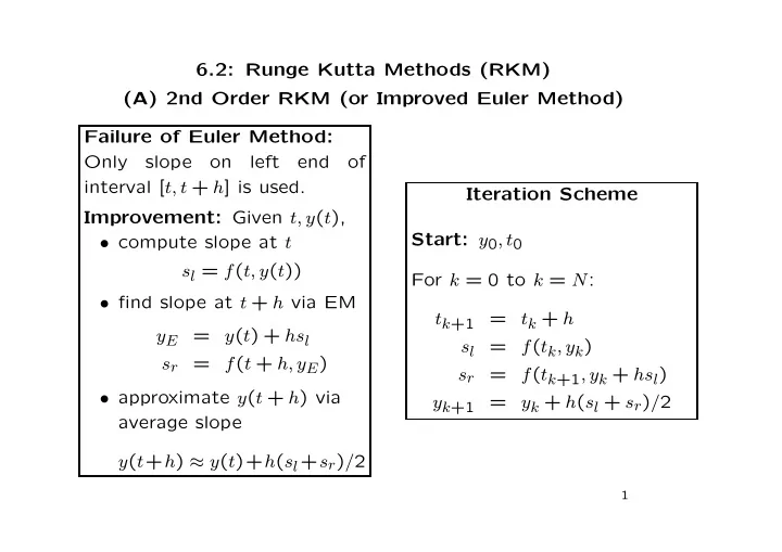
6.2: Runge Kutta Methods (RKM) (A) 2nd Order RKM (or Improved Euler Method) Failure of Euler Method: Only slope

• n

left end

• f

interval [t, t + h] is used. Improvement: Given t, y(t),

• compute slope at t

sl = f(t, y(t))

• find slope at t + h via EM

yE = y(t) + hsl sr = f(t + h, yE)

• approximate y(t + h) via

average slope y(t+h) ≈ y(t)+h(sl+sr)/2 Iteration Scheme Start: y0, t0 For k = 0 to k = N: tk+1 = tk + h sl = f(tk, yk) sr = f(tk+1, yk + hsl) yk+1 = yk + h(sl + sr)/2

1

• Ex. Approximate the solution to

y′ = t − y, y(0) = 0.5 in 0 ≤ t ≤ 1 using h = 0.25. Start: y0 = 0.5, t0 = 0 t1 = 0.25 sl = t0 − y0 = −0.5 sr = t1 − (y0 + hsl) = −0.125 y1 = y0 + h(sl + sr)/2 = 0.4219 t2 = 0.5 sl = t1 − y1 = −0.1719 sr = t2 − (y1 + hsl) = 0.1211 y2 = y1 + h(sl + sr)/2 = 0.4155 t3 = 0.75 sl = t2 − y2 = 0.0845 sr = t3 − (y2 + hsl) = 0.3134 y3 = y2 + h(sl + sr)/2 = 0.4653 t4 = 1 sl = t3 − y3 = 0.0845 sr = t4 − (y3 + hsl) = 0.3134 y4 = y3 + h(sl + sr)/2 = 0.4653 Ex.: y′ = t − y, y(0) = 0.5 Approximate y(1) for stepsizes h = 1/m, m = 1, 2, 4, 8, 16, 32 Exact Value: y(1) = 0.551819 Error: E(h) = |y(1) − ym| h ym E(h) 1 0.75 0.198181 1/2 0.585938 0.034118 1/4 0.558794 0.006974 1/8 0.553400 0.001581 1/16 0.552196 0.000377 1/32 0.551911 0.000092 E(h/2) ≈ E(h)/4 ⇒ E(h) ≈ C h2

Theorem: There ∃ C > 0 s.t. E(h) ≤ C h2 (2nd order RKM is second

• rder method)

2

(B) 4th Order RKM Idea: Given t and y = y(t), compute slopes s1, s2, s3, s4 at four carefully chosen points s.t. error is minimized. Approximation: y(t+h) ≈ y+h 6(s1+2s2+2s3+s4) Iteration k → k + 1: s1 = f(tk, yk) s2 = f(tk + h/2, yk + hs1/2) s3 = f(tk + h/2, yk + hs2/2) s4 = f(tk + h, yk + hs3) yk+1 = yk + h 6(s1 + 2s2 + 2s3 + s4) tk+1 = tk + h

Ex.: y′ = t−y, y(0) = 0.5, y(1) ≈ ym m = 1, 2, 4, 8, 16, 32, h = 1/m Exact Value: y(1) = 0.551819162 Error: E(h) = |y(1) − ym| h ym E(h) 1 0.5625 0.010680838 1/2 0.552256266 0.000437105 1/4 0.551841299 0.000022137 1/8 0.551820408 0.000001246 1/16 0.551819236 0.000000074 1/32 0.551819166 0.000000005 E(h/2) ≈ E(h)/16 ⇒ E(h) ≈ C h4

Theorem: There ∃ C > 0 s.t. E(h) ≤ C h4 (4th order RKM is fourth

• rder method)

3

Error Comparison

• Ex. y′ = t − y, y(0) = 0.5

y(1) ≈ ym → E(h) = |y(1) − ym| h = 1/m, m = 1, 2, 4, 8, 16, 32 h EM RKM2 RKM4 1 0.5518 0.198181 0.010680838 1/2 0.1768 0.034118 0.000437105 1/4 0.0772 0.006974 0.000022137 1/8 0.0364 0.001581 0.000001246 1/16 0.0177 0.000377 0.000000074 1/32 0.0087 0.000092 0.000000005 E(h) for EM: Euler Method RKM2: 2nd order RKM RKM4: 4th order RKM

Least square fit of E(h)

0.1 0.2 0.3 0.4 0.5 0.05 0.1 0.15

h E(h) EM RK2 EM: E(h)≈0.3412 h RK2: E(h)≈0.1348 h2

0.1 0.2 0.3 0.4 0.5 1 2 3 4 x 10

−4

h E(h) RK4: E(h)≈0.0070 h4

4

Worked out Examples from Exercises

• Ex. 3: y′ = ty, y(0) = 1.

Compute five RK2-iterates for h = 0.1. Arrange computation and results in a table. k tk yk sl sr h h(sl + sr)/2 1 0.1 0.1 0.005 1 0.1 1.0050 0.1005 0.2030 0.1 0.0152 2 0.2 1.0202 0.2040 0.3122 0.1 0.0258 3 0.3 1.0460 0.3138 0.4309 0.1 0.0372 4 0.4 1.0832 0.4333 0.5633 0.1 0.0498 5 0.5 1.1331 0.5665 0.7138 0.1 0.0640

5

• Ex. 7: z′ + z = cos x, z(0) = 1

(i) Compute RK2-approximations in 0 ≤ x ≤ 1 for h = 0.2, h = 0.1, h = 0.05. (ii) Find exact solution (iii) Plot exact solution as curve and RK2 approximations as points. (i) In Matlab, the RK2 approximation for h = 0.2 is computed and stored in arrays x0 2, z0 2 via h=0.2; m=1/h;x=0;z=1; xv=x;zv=z; for k=1:m sl=cos(x)-z; sr=cos(x+h)-(z+sl*h); z=z+h*(sl+sr)/2;zv=[zv z]; x=x+h;xv=[xv x]; end x0_2=xv;z0_2=zv; Analogously for h = 0.1 and h = 0.05 (arrays x0 1, z0 1 and x0 05, z0 05). (ii) Variation of Parameter: z′

h = −z ⇒ zh(x) = e−x

z(x) = e−x +

x

eξ cos(ξ) dξ = (cos x + sin x + e−x)/2 (iii) Plot: (see CN Sec. 6.1 for commands)

0.2 0.4 0.6 0.8 1 0.86 0.88 0.9 0.92 0.94 0.96 0.98 1

x z

• : h=0.2

*: h=0.1 +: h=0.05

6

• Ex. 7a: z′ + z = cos x, z(0) = 1

(i) Compute RK4-approximation in 0 ≤ x ≤ 1 for h = 0.2. (iii) Plot exact solution as curve and RK4 approximation as points. (i) RK4 approximation for h = 0.2 is computed and stored in arrays xv, zv: h=0.2; m=1/h;x=0;z=1; xv=x;zv=z; for k=1:m s1=cos(x)-z; s2=cos(x+h/2)-(z+s1*h/2); s3=cos(x+h/2)-(z+s2*h/2); s4=cos(x+h)-(z+s3*h); z=z+h*(s1+2*s2+2*s3+s4)/6; zv=[zv z]; x=x+h;xv=[xv x]; end (iii) Matlab plot commands: x=linspace(0,1,100); z=1/2*(cos(x)+sin(x)+exp(-x)); plot(xv,zv,’ko’,x,z,’k’), xlabel(’x’),ylabel(’z’), axis([0 1 0.86 1])

0.2 0.4 0.6 0.8 1 0.86 0.88 0.9 0.92 0.94 0.96 0.98 1

x z

7