5. Linear Inequalities and Elimination Searching for certificates - PowerPoint PPT Presentation

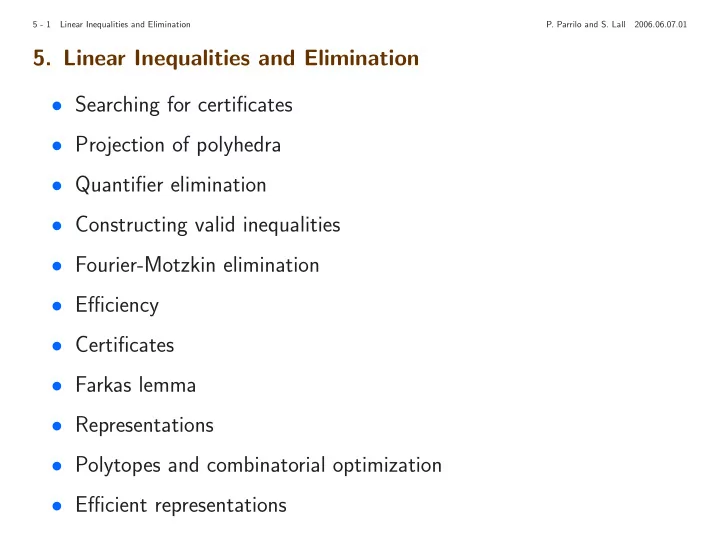
5 - 1 Linear Inequalities and Elimination P. Parrilo and S. Lall 2006.06.07.01 5. Linear Inequalities and Elimination • Searching for certificates • Projection of polyhedra • Quantifier elimination • Constructing valid inequalities • Fourier-Motzkin elimination • Efficiency • Certificates • Farkas lemma • Representations • Polytopes and combinatorial optimization • Efficient representations

5 - 2 Linear Inequalities and Elimination P. Parrilo and S. Lall 2006.06.07.01 Searching for Certificates Given a feasibility problem does there exist x such that f i ( x ) ≤ 0 for all i = 1 , . . . , m We would like to find certificates of infeasibility. Two important methods include • Optimization • Automated inference, or constructive methods In this section, we will describe some constructive methods for the special case of linear equations and inequalities

5 - 3 Linear Inequalities and Elimination P. Parrilo and S. Lall 2006.06.07.01 Polyhedra A set S ⊂ R n is called a polyhedron if it is the intersection of a finite set of closed halfspaces x ∈ R n | Ax ≤ b � � S = • A bounded polyhedron is called a polytope • The dimension of a polyhedron is the dimension of its affine hull � � affine ( S ) = λx + νy | λ + ν = 1 , x, y ∈ S • If b = 0 the polyhedron is a cone • Every polyhedron is convex

5 - 4 Linear Inequalities and Elimination P. Parrilo and S. Lall 2006.06.07.01 Faces of Polyhedra given a ∈ R n , the corresponding face of polyhedron P is � � x ∈ P | a T x ≥ a T y for all y ∈ P face ( a, P ) = � T , P ) , dimension 1 � face ( 1 1 � T , P ) , dimension 0 � face ( 2 1 • Faces of dimension 0 are called vertices 1 edges d − 1 facets , where d = dim( P ) • Facets are also said to have codimension 1

5 - 5 Linear Inequalities and Elimination P. Parrilo and S. Lall 2006.06.07.01 Projection of Polytopes Suppose we have a polytope x ∈ R n | Ax ≤ b � � S = We’d like to construct the projection onto the hyperplane � x ∈ R n | x 1 = 0 � Call this projection P ( S ) In particular, we would like to find the inequalities that define P ( S )

5 - 6 Linear Inequalities and Elimination P. Parrilo and S. Lall 2006.06.07.01 Projection of Polytopes We have � � x 1 � � P ( S ) = x 2 | there exists x 1 such that ∈ S x 2 • Our objective is to perform quantifier elimination to remove the exis- tential quantifier and find a basic semialgebraic representation of P ( S ) • Alternatively, we can interpret this as finding valid inequalities that do not depend on x 1 ; i.e., the intersection cone { f 1 , . . . , f m } ∩ R [ x 2 , . . . , x n ] This is called the elimination cone of valid inequalities

5 - 7 Linear Inequalities and Elimination P. Parrilo and S. Lall 2006.06.07.01 Projection of Polytopes • Intuitively, P ( S ) is a polytope; what are its vertices? Every face of P ( S ) is the projection of a face of S • Hence every vertex of P ( S ) is the projection of some vertex of S • What about the facets? • So one algorithm is • Find the vertices of S , and project them • Find the convex hull of the projected points But how do we do this?

5 - 8 Linear Inequalities and Elimination P. Parrilo and S. Lall 2006.06.07.01 Example • The polytope S has dimension 55, 2048 vertices, billions of facets • The 3d projection P ( S ) has 92 vertices and 74 facets

5 - 9 Linear Inequalities and Elimination P. Parrilo and S. Lall 2006.06.07.01 Simple Example 5 − 4 x 1 − x 2 ≤ − 9 (1) 7 4 5 − x 1 − 2 x 2 ≤ − 4 (2) 3 − 2 x 1 + x 2 ≤ 0 (3) 3 − x 2 − 6 x 2 ≤ − 6 (4) 2 1 6 x 1 + 2 x 2 ≤ 11 (5) 6 x 1 + 2 x 2 ≤ 17 (6) 1 x 2 ≤ 4 (7) 2 1 2 3 4 5

5 - 10 Linear Inequalities and Elimination P. Parrilo and S. Lall 2006.06.07.01 Constructing Valid Inequalities We can generate new valid inequalities from the given set; e.g., if a T a T 1 x ≤ b 1 and 2 x ≤ b 2 then λ 1 ( b 1 − a T 1 x ) + λ 2 ( b 2 − a T 2 x ) ≥ 0 is a valid inequality for all λ 1 , λ 2 ≥ 0 Here we are applying the inference rule, for λ 1 , λ 2 ≥ 0 f 1 , f 2 ≥ 0 ⇒ λ 1 f 1 + λ 2 f 2 ≥ 0 =

5 - 11 Linear Inequalities and Elimination P. Parrilo and S. Lall 2006.06.07.01 Constructing Valid Inequalities For example, use inequalities (2) and (6) above − x 1 + 2 x 2 ≤ − 4 6 x 1 − 2 x 2 ≤ 17 Pick λ 1 = 6 and λ 2 = 1 to give 6( − x 1 − 2 x 2 ) + (6 x 1 − 2 x 2 ) ≤ 6( − 4) + 17 − 2 x 2 ≤ 1 • The corresponding vector is in the cone generated by a 1 and a 2 • If a 1 and a 2 have opposite sign coefficients of x 1 , then we can pick some element of the cone with x 1 coefficient zero.

5 - 12 Linear Inequalities and Elimination P. Parrilo and S. Lall 2006.06.07.01 Fourier-Motzkin Elimination Write the original inequalities as  x 2 4 + 9   4     − 2 x 2 − 11  − 2 x 2 + 4    ≤ x 1 ≤ − x 2 3 + 17 x 2   6  2      − 6 x 2 + 6  along with x 2 ≤ 4 Hence every expression on the left hand side is less than every expression on the right, for every ( x 1 , x 2 ) ∈ P Together with x 2 ≤ 4 , this set of pairs specifies exactly P ( S )

5 - 13 Linear Inequalities and Elimination P. Parrilo and S. Lall 2006.06.07.01 The Projected Set This gives the following system of inequalities for P ( S ) − x 2 ≤ − 1 x 2 ≤ 4 2 x 2 ≤ 5 − x 2 ≤ 1 0 ≤ 7 5 2 − x 2 ≤ 4 − x 2 ≤ − 1 x 2 ≤ 17 x 2 ≤ 4 5 2 • There are many redundant inequalities • P ( S ) is defined by the tightest pair − x 2 ≤ − 1 x 2 ≤ 4 2 • When performing repeated projection, it is very important to eliminate redundant inequalities

5 - 14 Linear Inequalities and Elimination P. Parrilo and S. Lall 2006.06.07.01 Efficiency of Fourier-Motzkin elimination If A has m rows, then after elimination of x 1 we can have no more than � m 2 � facets 4 • If m/ 2 inequalities have a positive coefficient of x 1 , and m/ 2 have a negative coefficient, then FM constructs exactly m 2 / 4 new inequalities • Repeating this, eliminating d dimensions gives � 2 d � m inequalities 2 • Key question: how many are redundant? i.e., does projection produce exponentially more facets?

5 - 15 Linear Inequalities and Elimination P. Parrilo and S. Lall 2006.06.07.01 Inequality Representation Constructing such inequalities corresponds to multiplication of the original constraint Ax ≤ b by a positive matrix C In this case   1 0 0 0 4 0 0     6 0 0 0 0 4 0 − 4 − 1 − 9     0 1 0 0 1 0 0 − 1 − 2 − 4             0 6 0 0 0 1 0 − 2 1 0             C = 0 0 1 0 2 0 0 A = − 1 − 6 b = − 6             0 0 6 0 0 2 0 1 2 11             0 0 0 1 1 0 0 6 − 2 17         0 0 0 6 0 1 0 0 1 4   0 0 0 0 0 0 1

5 - 16 Linear Inequalities and Elimination P. Parrilo and S. Lall 2006.06.07.01 Inequality Representation The resulting inequality system is CAx ≤ Cb , since x ≥ 0 and C ≥ 0 ⇒ Cx ≥ 0 = We find     0 7 35 0 − 14 14         0 0 7         0 − 14 − 7         CA = 0 5 Cb = 22         0 2 34         0 − 4 5         0 − 38 − 19     0 1 4

5 - 17 Linear Inequalities and Elimination P. Parrilo and S. Lall 2006.06.07.01 Feasibility In the example above, we eliminated x 1 to find − x 2 ≤ − 1 x 2 ≤ 4 2 We can now eliminate x 2 to find 0 ≤ 7 2 which is obviously true; it’s valid for every x ∈ S , but happens to be independent of x If we had arrived instead at 0 ≤ − 2 then we would have derived a contradiction, and the original system of inequalities would therefore be infeasible

5 - 18 Linear Inequalities and Elimination P. Parrilo and S. Lall 2006.06.07.01 Example Consider the infeasible system x 1 ≥ 0 x 2 ≥ 0 x 1 + x 2 ≤ − 2 Write this as − x 1 ≤ 0 x 1 + x 2 ≤ − 2 − x 2 ≤ 0 Eliminating x 1 gives x 2 ≤ − 2 − x 2 ≤ 0 Subsequently eliminating x 2 gives the contradiction 0 ≤ − 2

5 - 19 Linear Inequalities and Elimination P. Parrilo and S. Lall 2006.06.07.01 Inequality Representation     − 1 0 0  and b = The original system is Ax ≤ b with A = 1 1 − 2    0 − 1 0 To eliminate x 1 , multiply � 1 1 0 � ( Ax − b ) ≤ 0 0 0 1 Similarly to eliminate x 2 we form � � 1 1 0 � � 1 1 ( Ax − b ) ≤ 0 0 0 1

5 - 20 Linear Inequalities and Elimination P. Parrilo and S. Lall 2006.06.07.01 Certificates of Infeasibility The final elimination is � � 1 1 1 ( Ax − b ) ≤ 0 Hence we have found a vector λ such that • λ ≥ 0 (since its a product of positive matrices) • λ T A = 0 and λ T b < 0 (since it gives a contradiction) Fourier-Motzkin constructs a certificate of infeasibility; the vector λ • Exactly decides feasibility of linear inequalities • Hence this gives an extremely inefficient way to solve a linear program