
SLIDE 1
1
Auctions, Negotiations
R&N, 17.6
6,?? 0,??
- 4,??
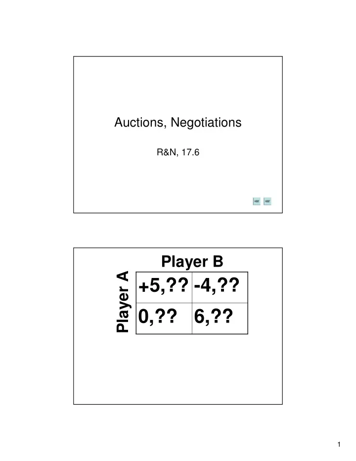
+5,?? -4,?? 0,?? 6,?? 1 Player B +5,?? -4,?? Player A 0,?? - - PDF document
Auctions, Negotiations R&N, 17.6 Player B Player A +5,?? -4,?? 0,?? 6,?? 1 Player B +5,?? -4,?? Player A 0,?? 6,?? So far, we have assumed that both players know exactly the payoffs they get for every pair of pure strategies
1
R&N, 17.6
2
the payoffs they get for every pair of pure strategies
the payoffs for Player B?
making scenarios. When does this situation arise?
watch hockey games but B prefers to go see a
alone; each would rather go the other’s preferred choice rather than go alone to its own.
3
watch hockey games but B prefers to go see a
alone; each would rather go the other’s preferred choice rather than go alone to its own.
share the activity with B; but he is not sure that B wants to sure the activity A does not know B’s payoff structure.
4
know probabilities for each of B’s preferences In this example, A may know how likely it is that B wants to meet/avoid him
having different types.
“wishes to meet” or “wishes to avoid”
type of each player denoted by tA and tB
that the player A has type tA, assuming the player B has type tB, for all possible pairs of values of tA and tB.
– P(tA|tB) Belief of player A’s type given player B’s type – P(tB|tA) Belief of player B’s type given player A’s type
5
P(tA=meet | tB=meet) = 1 P(tA=meet | tB=avoid) = 1 P(tA=avoid | tB=meet) = 0 P(tA=avoid | tB=avoid) = 0 P(tB=meet | tA=meet) = 1/2 P(tB=meet | tA=avoid) = 1/2 P(tB=avoid | tA=meet) = 1/2 P(tB=avoid | tA=avoid) = 1/2
sA(tA)
is, what is the expected payoff for Player A?
type tA is the sum of the payoffs he would receive for each possible type from the other player, weighted by the probability that the other player is in that type.
B Player
types possible all A B t B B A A A A
B
6
B Player
types possible all A B t B B A A A A
B
Payoff if Player A knows that Player B is of type tB Probability that Player B is indeed of type tB Since Player A does not know Player B’s type, it has to sum over all possible types to get the expected value
+1,+2 0,0 Movie 0,0 +2,+1 Hockey Movie Hockey +1,0 0,+1 Movie 0,+2 +2,0 Hockey Movie Hockey
7
Expected payoff to Player A if he chooses H and Player B chooses:
be (finally) extended to this case.
payoffs by the expected payoff for each type of player
for all possible types tA and tB is an equilibrium if
) | P( ) ( ), ( max arg ) (
B Player
types possible all * * A B t B B A A A s A
t t t s t s u t s
B A A
) | P( ) ( ), ( max arg ) (
A Player
types possible all * * B A t B B A A B s B
t t t s t s u t s
A B B
8
) | P( ) ( ), ( max arg ) (
B Player
types possible all * * A B t B B A A A s A
t t t s t s u t s
B A A
Assuming Player B’s uses s*B(tB) for all types tB Player A cannot get higher payoff than by playing s*A(tA) : s*A(tA) is the best that Player A can achieve
equilibrium as before but for the “supergame” with as many players as there are pairs (Player,Type) and with the definition of the expected payoffs
the best strategy for rational players given their beliefs about the other players’ state
+1,+2 0,0 Movie 0,0 +2,+1 Hockey Movie Hockey +1,0 0,+1 Movie 0,+2 +2,0 Hockey Movie Hockey
9
+1,+2 0,0 Movie 0,0 +2,+1 Hockey Movie Hockey +1,0 0,+1 Movie 0,+2 +2,0 Hockey Movie Hockey
The strategy: S*A = H S*B=
Is the equilibrium because:
B B B A B B A B A A B A A B A A
t s s s u s s u t s s s u s s u ∀ ∀ ≥ ∀ ∀ ≥ ) , ( ) , ( ) , ( ) , (
* * * * * *
10
expected payoffs are termed Bayesian Games.
extend directly to n players (albeit with considerably more painful notations)
) | P( ) ( , , ), ( max arg ) (
) (not Players
the
types possible all * 1 * 1 * i i i t n n i A s i
t t t s s t s u t s
i i i
−
=
= types of all the players except i
for sale
knows, but none of the other buyers know): Vi in [0,1]
assumes that the Vj’s are randomly (uniformly) drawn from [0,1]
the other buyers follow the best (rational) strategy?
11
price = bid gio
(“Dutch”) auctions.
= bid gio
Player i
– Vi – gi if gi = maxj(gj) – 0 otherwise
mentioning the problem of the ties (gi = gj for 2 different players), tie- breaking rules must be built into the auction
12
= bid gio
Player i
– Vi – gi if gi = maxj(gj) – 0 otherwise
– Types are the different values Vi for each player i – Player j does not know the value Vi for player i, but it knows the belief distribution for this value (uniform in this case)
reached for: g*i = argmaxg (Expected payoff for player i)
13
reached for: g*i = argmaxg (Expected payoff for player i bidding g)
auction, so: g*i = argmaxg (Expected payoff for player i bidding g when i wins) x Prob(i wins)
is of the form:
all the other Players j
depend on Player i and it is unimportant
14
reached for: g*i = argmaxg (Expected payoff for player i bidding g)
auction, so: g*i = argmaxg (Expected payoff for player i bidding g when i wins x Prob(i wins))
= Prob(g > all of the other n-1 bids) proportional to gn-1 = (Vi-g)
reached for: g*i = argmaxg (Expected payoff for player i bidding g when i wins x Prob(i wins)) g*i = argmaxg (Vi-g) gn-1
derivative is zero:
15
the max of n numbers randomly and uniformly drawn from [0,1] is n/(n+1)
16
price = second highest bid
Player i
– Vi – go if gi = maxj(gj) go = max j neq i (gj) – 0 otherwise
mentioning the problem of the ties (gi = gj for 2 different players), tie- breaking rules must be built into the auction
17
(maximum payoff). In particular, gi = Vi wins.
(maximum payoff is 0). In particular, gi = Vi loses.
irrespective of the other players’ bids
equilibrium is: g*i = Vi
– S assigns a value VS to the object – B assigns a value VB to the object – Neither player knows the other player’s assigned value, but they both know a distribution over the values (for example, drawn randomly and uniformly from [0 1])
receives the object
– S Payoff = (gS + gB)/2 – VS – B Payoff = VB - (gS + gB)/2
18
formalism as before:
– Players: S and B – Types: The values VS and VB in [0 1] – Actions: The bids gS and gB in [0 1] – Beliefs: Uniform distribution on [0 1] for VS and VB
uS = Expected payoff to S = (Expected payoff to S if trade occurs) x Prob(trade occurs) = (Expected payoff to S if trade occurs) x Prob(gB > gS)
– g*B(VB)= 1/12 + 2/3 VB – g*S(VS)= 1/4 + 2/3 VS
¼ ½ ¾ 1
19
be used to analyze auctions
economics (e.g., auction of radio spectrum…); it is becoming increasingly important for the design of autonomous agents
– Cooperative auctions – Many goods – Other mechanisms (time limits, multiple bids, etc.) – Risk adverse buyers – Non-uniform beliefs
which the payoffs are uncertain
cases by introducing the notion of “player type” and by replacing playoffs by “expected payoffs” computed using beliefs over player types (e.g., probability that Player B wants to meet Player A)
– First-price auctions – Second-price auctions – Double auction negotiation