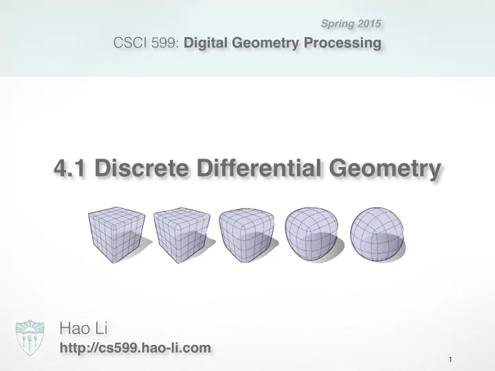
4 1 discrete differential geometry
play

4.1 Discrete Differential Geometry Hao Li http://cs599.hao-li.com - PowerPoint PPT Presentation

Spring 2015 CSCI 599: Digital Geometry Processing 4.1 Discrete Differential Geometry Hao Li http://cs599.hao-li.com 1 Outline Discrete Differential Operators Discrete Curvatures Mesh Quality Measures 2 Differential Operators on


  1. Spring 2015 CSCI 599: Digital Geometry Processing 4.1 Discrete Differential Geometry Hao Li http://cs599.hao-li.com 1

  2. Outline • Discrete Differential Operators • Discrete Curvatures • Mesh Quality Measures 2

  3. Differential Operators on Polygons Differential Properties � • Surface is sufficiently differentiable • Curvatures → 2nd derivatives 3

  4. Differential Operators on Polygons Differential Properties � • Surface is sufficiently differentiable • Curvatures → 2nd derivatives Polygonal Meshes � • Piecewise linear approximations of smooth surface • Focus on Discrete Laplace Beltrami Operator • Discrete differential properties defined over N ( x ) 4

  5. Local Averaging N ( x ) Local Neighborhood of a point � x • often coincides with mesh vertex v i N n ( v i ) • n-ring neighborhood or local geodesic ball 5

  6. Local Averaging N ( x ) Local Neighborhood of a point � x • often coincides with mesh vertex v i N n ( v i ) • n-ring neighborhood or local geodesic ball Neighborhood size � • Large: smoothing is introduced, stable to noise • Small: fine scale variation, sensitive to noise 6

  7. Local Averaging: 1-Ring N ( x ) x Barycentric cell Voronoi cell Mixed Voronoi cell (barycenters/edgemidpoints) (circumcenters) (circumcenters/midpoint) tight error bound better approximation 7

  8. Barycentric Cells Connect edge midpoints and triangle barycenters � • Simple to compute • Area is 1/3 o triangle areas • Slightly wrong for obtuse triangles 8

  9. Mixed Cells Connect edge midpoints and � • Circumcenters for non-obtuse triangles • Midpoint of opposite edge for obtuse triangles • Better approximation, more complex to compute… 9

  10. Normal Vectors Continuous surface   x ( u, v ) y ( u, v ) x ( u, v ) =   z ( u, v ) n Normal vector x u x v p x u � x v n = ⇥ x u � x v ⇥ Assume regular parameterization x u � x v ⇥ = 0 normal exists 10

  11. Discrete Normal Vectors n ( T ) x k x i x j 11

  12. Discrete Normal Vectors n ( v ) n ( T ) x k x i x j 12

  13. Discrete Normal Vectors n ( v ) n ( T ) x k x i θ T x j 13

  14. Discrete Normal Vectors tessellated cylinder 14

  15. Simple Curvature Discretization mean curvature ∆ S x = div S ∇ S x = − 2 H n Laplace-Beltrami 15

  16. Simple Curvature Discretization mean curvature ∆ S x = div S ∇ S x = − 2 H n Laplace-Beltrami How to discretize? 16

  17. Laplace Operator on Meshes Extend finite differences to meshes? � • What weights per vertex/edge? ¼ ? ? ? ? ¼ ? ¼ -1 ½ -1 ½ ? ? ¼ 1D grid 2D grid 2D/3D grid 17

  18. Uniform Laplace Uniform discretization � • What weights per vertex/edge? Properties � • depends only on connectivity • simple and efficient 18

  19. Uniform Laplace Uniform discretization � 1 � ∆ uni x i := ( x j − x i ) ≈ − 2 H n |N 1 ( v i ) | v j ∈ N 1 ( v i ) Properties � • depends only on connectivity • simple and efficient • bad approximation for irregular triangulations • can give non-zero for planar meshes H • tangential drift for mesh smoothing 19

  20. Gradients mean curvature ∆ S x = div S ∇ S x = − 2 H n Laplace-Beltrami gradient operator Discrete Gradient of a Function � • Defined on piecewise linear triangle • Important for parameterization and deformation 20

  21. Gradients x k x i triangle x j u = ( u, v ) piecewise linear function f i = f ( x i ) linear basis functions for barycentric interpolation on a triangle 21

  22. Gradients u = ( u, v ) piecewise linear function 22

  23. Gradients u = ( u, v ) piecewise linear function gradient of linear function 23

  24. Gradients u = ( u, v ) piecewise linear function gradient of linear function partition of unity gradients of basis 24

  25. Gradients u = ( u, v ) piecewise linear function gradient of linear function partition of unity gradients of basis gradient of linear function 25

  26. Gradients gradient of linear function

  27. Gradients gradient of linear function with appropriate normalization: 27

  28. Gradients gradient of linear function with appropriate normalization: f i = f ( x i ) discrete gradient of a piecewiese linear function within T 28

  29. Discrete Laplace-Beltrami gradient mean operator curvature ∆ S x = div S ∇ S x = − 2 H n Laplace-Beltrami

  30. Discrete Laplace-Beltrami gradient mean operator curvature ∆ S x = div S ∇ S x = − 2 H n Laplace-Beltrami divergence theorem 30

  31. Discrete Laplace-Beltrami gradient mean operator curvature ∆ S x = div S ∇ S x = − 2 H n Laplace-Beltrami divergence theorem vector-valued function local averaging domain boundary 31

  32. Discrete Laplace-Beltrami gradient mean operator curvature ∆ S x = div S ∇ S x = − 2 H n Laplace-Beltrami divergence theorem 32

  33. Discrete Laplace-Beltrami average Laplace-Beltrami 33

  34. Discrete Laplace-Beltrami average Laplace-Beltrami gradient is constant and local Voronoi passes through a,b: over triangle 34

  35. Discrete Laplace-Beltrami average Laplace-Beltrami gradient is constant and local Voronoi passes through a,b: over triangle discrete gradient 35

  36. Discrete Laplace-Beltrami average Laplace-Beltrami within a triangle 36

  37. Discrete Laplace-Beltrami average Laplace-Beltrami within a triangle 37

  38. Discrete Laplace-Beltrami average Laplace-Beltrami over averaging region 38

  39. Discrete Laplace-Beltrami average Laplace-Beltrami over averaging region discrete Laplace-Beltrami 39

  40. Discrete Laplace-Beltrami Cotangent discretization � 1 � ∆ S f ( v i ) := (cot α ij + cot β ij ) ( f ( v j ) − f ( v i )) 2 A ( v i ) v j ∈ N 1 ( v i ) A ( v i ) v i β ij α ij for full derivation, check out: http://brickisland.net/cs177/ v j 40

  41. Discrete Laplace-Beltrami Cotangent discretization 1 � ∆ S f ( v ) := (cot α i + cot β i ) ( f ( v i ) − f ( v )) 2 A ( v ) v i ∈ N 1 ( v ) Problems � • weights can become negative • depends on triangulation Still the most widely used discretization 41

  42. Outline • Discrete Differential Operators • Discrete Curvatures • Mesh Quality Measures 42

  43. Discrete Curvatures How to discretize curvature on a mesh? � • Zero curvature within triangles • Infinite curvature at edges / vertices • Point-wise definition doesn’t make sense Approximate differential properties at point as x average over local neighborhood � A ( x ) • is a mesh vertex A ( x ) x • within one-ring neighborhood A ( x ) x 43

  44. Discrete Curvatures How to discretize curvature on a mesh? � • Zero curvature within triangles • Infinite curvature at edges / vertices • Point-wise definition doesn’t make sense Approximate differential properties at point as x average over local neighborhood A ( x ) A ( x ) 1 � K ( v ) ≈ K ( x ) d A A ( v ) ( v ) A x 44

  45. Discrete Curvatures Which curvatures to discretize? � • Discretize Laplace-Beltrami operator • Laplace-Beltrami gives us mean curvature H • Discretize Gaussian curvature K • From and we can compute and H K κ 2 κ 1 mean curvature ∆ S x = div S ∇ S x = − 2 H n Laplace-Beltrami 45

  46. Discrete Gaussian Curvature Gauss-Bonnet Z K = 2 πχ χ = 2 − 2 g Discrete Gauss Curvature � K = (2 π − θ j ) /A j Verify via Euler-Poincaré V − E + F = 2(1 − g ) 46

  47. Discrete Curvatures Mean curvature (absolute value) H = 1 2 � ∆ S x � A Gaussian curvature � K = (2 π − θ j ) /A θ j j Principal curvatures � � H 2 − K H 2 − K κ 1 = H + κ 2 = H − 47

  48. Outline • Discrete Differential Operators • Discrete Curvatures • Mesh Quality Measures 48

  49. Mesh Quality Visual inspection of “sensitive” attributes � • Specular shading 49

  50. Mesh Quality Visual inspection of “sensitive” attributes � • Specular shading • Reflection lines 50 50

  51. Mesh Quality Visual inspection of “sensitive” attributes � • Specular shading • Reflection lines • differentiability one order lower than surface • can be efficiently computed using GPU C 0 C 1 C 2 51 51 51

  52. Mesh Quality Visual inspection of “sensitive” attributes � • Specular shading • Reflection lines • Curvature • Mean curvature 52

  53. Mesh Quality Visual inspection of “sensitive” attributes � • Specular shading • Reflection lines • Curvature • Gauss curvature 53

  54. Mesh Quality Criteria Smoothness � • Low geometric noise 54

  55. Mesh Quality Criteria Smoothness � • Low geometric noise Fairness � • Simplest shape 55

  56. Mesh Quality Criteria Smoothness � • Low geometric noise Fairness � • Simplest shape Adaptive tesselation � • Low complexity 56

  57. Mesh Quality Criteria Smoothness � • Low geometric noise Fairness � • Simplest shape Adaptive tesselation � • Low complexity Triangle shape � • Numerical Robustness 57

  58. Mesh Optimization Smoothness � • Smoothing Fairness � • Fairing Adaptive tesselation � • Decimation Triangle shape � • Remeshing 58

Download Presentation
Download Policy: The content available on the website is offered to you 'AS IS' for your personal information and use only. It cannot be commercialized, licensed, or distributed on other websites without prior consent from the author. To download a presentation, simply click this link. If you encounter any difficulties during the download process, it's possible that the publisher has removed the file from their server.

Recommend


More recommend