3 Language Models 1: n -gram Language Models While the final goal of - - PDF document

3 Language Models 1: n-gram Language Models

While the final goal of a probabilistic machine translation system is to create a model of the target sentence E given the source sentence F, P(E | F), in this chapter we will take a step back, and attempt to create a language model of only the target sentence P(E). Basically, this model allows us to do two things that are of practical use. Assess naturalness: Given a sentence E, this can tell us, does this look like an actual, natural sentence in the target language? If we can learn a model to tell us this, we can use it to assess the fluency of sentences generated by an automated system to improve its

• results. It could also be used to evaluate sentences generated by a human for purposes
• f grammar checking or error correction.

Generate text: Language models can also be used to randomly generate text by sampling a sentence E0 from the target distribution: E0 ⇠ P(E).4 Randomly generating samples from a language model can be interesting in itself – we can see what the model “thinks” is a natural-looking sentences – but it will be more practically useful in the context of the neural translation models described in the following chapters. In the following sections, we’ll cover a few methods used to calculate this probability P(E).

3.1 Word-by-word Computation of Probabilities

As mentioned above, we are interested in calculating the probability of a sentence E = eT

1 .

Formally, this can be expressed as P(E) = P(|E| = T, eT

1 ),

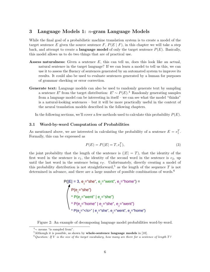
(3) the joint probability that the length of the sentence is (|E| = T), that the identity of the first word in the sentence is e1, the identity of the second word in the sentence is e2, up until the last word in the sentence being eT . Unfortunately, directly creating a model of this probability distribution is not straightforward,5 as the length of the sequence T is not determined in advance, and there are a large number of possible combinations of words.6

P(|E| = 3, e1=”she”, e2=”went”, e3=”home”) = P(e1=“she”) * P(e2=”went” | e1=“she”) * P(e3=”home” | e1=“she”, e2=”went”)

* P(e4=”</s>” | e1=“she”, e2=”went”, e3=”home”) Figure 2: An example of decomposing language model probabilities word-by-word.

4∼ means “is sampled from”. 5Although it is possible, as shown by whole-sentence language models in [10]. 6Question: If V is the size of the target vocabulary, how many are there for a sentence of length T?

6

i am from pittsburgh . i study at a university . my mother is from utah .

P(e2=am | e1=i) = c(e1=i, e2=am)/c(e1=i) = 1 / 2 = 0.5 P(e2=study | e1=i) = c(e1=i, e2=study)/c(e1=i) = 1 / 2 = 0.5 Figure 3: An example of calculating probabilities using maximum likelihood estimation. As a way to make things easier, it is common to re-write the probability of the full sen- tence as the product of single-word probabilities. This takes advantage of the fact that a joint probability – for example P(e1, e2, e3) – can be calculated by multiplying together con- ditional probabilities for each of its elements. In the example, this means that P(e1, e2, e3) = P(e1)P(e2 | e1)P(e3 | e1, e2). Figure 2 shows an example of this incremental calculation of probabilities for the sentence “she went home”. Here, in addition to the actual words in the sentence, we have introduced an implicit sentence end (“h/si”) symbol, which we will indicate when we have terminated the

• sentence. Stepping through the equation in order, this means we first calculate the probability
• f “she” coming at the beginning of the sentence, then the probability of “went” coming next

in a sentence starting with “she”, the probability of “home” coming after the sentence prefix “she went”, and then finally the sentence end symbol “h/si” after “she went home”. More generally, we can express this as the following equation: P(E) =

T+1

Y

t=1

P(et | et1

1

) (4) where eT+1 = h/si. So coming back to the sentence end symbol h/si, the reason why we introduce this symbol is because it allows us to know when the sentence ends. In other words, by examining the position of the h/si symbol, we can determine the |E| = T term in our

• riginal LM joint probability in Equation 3. In this example, when we have h/si as the 4th

word in the sentence, we know we’re done and our final sentence length is 3. Once we have the formulation in Equation 4, the problem of language modeling now becomes a problem of calculating the next word given the previous words P(et | et1

1

). This is much more manageable than calculating the probability for the whole sentence, as we now have a fixed set of items that we are looking to calculate probabilities for. The next couple

• f sections will show a few ways to do so.

3.2 Count-based n-gram Language Models

The first way to calculate probabilities is simple: prepare a set of training data from which we can count word strings, count up the number of times we have seen a particular string of words, and divide it by the number of times we have seen the context. This simple method, can be expressed by the equation below, with an example shown in Figure 3 PML(et | et1

1

) = cprefix(et

1)

cprefix(et1

1

). (5) 7

Here cprefix(·) is the count of the number of times this particular word string appeared at the beginning of a sentence in the training data. This approach is called maximum likelihood estimation (MLE, details later in this chapter), and is both simple and guaranteed to create a model that assigns a high probability to the sentences in training data. However, let’s say we want to use this model to assign a probability to a new sentence that we’ve never seen before. For example, if we want to calculate the probability of the sentence “i am from utah .” based on the training data in the example. This sentence is extremely similar to the sentences we’ve seen before, but unfortunately because the string “i am from utah” has not been observed in our training data, cprefix(i, am, from, utah) = 0, P(e4 = utah | e1 = i, e2 = am, e3 = from) becomes zero, and thus the probability of the whole sentence as calculated by Equation 5 also becomes zero. In fact, this language model will assign a probability of zero to every sentence that it hasn’t seen before in the training corpus, which is not very useful, as the model loses ability to tell us whether a new sentence a system generates is natural or not, or generate new outputs. To solve this problem, we take two measures. First, instead of calculating probabilities from the beginning of the sentence, we set a fixed window of previous words upon which we will base our probability calculations, approximating the true probability. If we limit our context to n 1 previous words, this would amount to: P(et | et1

1

) ⇡ PML(et | et1

tn+1).

(6) Models that make this assumption are called n-gram models. Specifically, when models where n = 1 are called unigram models, n = 2 bigram models, n = 3 trigram models, and n 4 four-gram, five-gram, etc. The parameters θ of n-gram models consist of probabilities of the next word given n 1 previous words: θet

t−n+1 = P(et | et1

tn+1),

(7) and in order to train an n-gram model, we have to learn these parameters from data.7 In the simplest form, these parameters can be calculated using maximum likelihood estimation as follows: θet

t−n+1 = PML(et | et1

tn+1) = c(et tn+1)

c(et1

tn+1),

(8) where c(·) is the count of the word string anywhere in the corpus. Sometimes these equations will reference etn+1 where t n + 1 < 0. In this case, we assume that etn+1 = hsi where hsi is a special sentence start symbol. If we go back to our previous example and set n = 2, we can see that while the string “i am from utah .” has never appeared in the training corpus, “i am”, “am from”, “from utah”, “utah .”, and “. h/si” are all somewhere in the training corpus, and thus we can patch together probabilities for them and calculate a non-zero probability for the whole sentence.8 However, we still have a problem: what if we encounter a two-word string that has never appeared in the training corpus? In this case, we’ll still get a zero probability for that particular two-word string, resulting in our full sentence probability also becoming zero. n- gram models fix this problem by smoothing probabilities, combining the maximum likelihood

7Question: How many parameters does an n-gram model with a particular n have? 8Question: What is this probability?

8

estimates for various values of n. In the simple case of smoothing unigram and bigram probabilities, we can think of a model that combines together the probabilities as follows: P(et | et1) = (1 α)PML(et | et1) + αPML(et), (9) where α is a variable specifying how much probability mass we hold out for the unigram

• distribution. As long as we set α > 0, regardless of the context all the words in our vocabulary

will be assigned some probability. This method is called interpolation, and is one of the standard ways to make probabilistic models more robust to low-frequency phenomena. If we want to use even more context – n = 3, n = 4, n = 5, or more – we can recursively define our interpolated probabilities as follows: P(et | et1

tm+1) = (1 αm)PML(et | et1 tm+1) + αmP(et | et1 tm+2).

(10) The first term on the right side of the equation is the maximum likelihood estimate for the model of order m, and the second term is the interpolated probability for all orders up to m 1. There are also more sophisticated methods for smoothing, which are beyond the scope of this section, but summarized very nicely in [4]. Context-dependent smoothing coefficients: Instead of having a fixed α, we condition the interpolation coefficient on the context: αet−1

t−m+1. This allows the model to give

more weight to higher order n-grams when there are a sufficient number of training examples for the parameters to be estimated accurately and fall back to lower-order n-grams when there are fewer training examples. These context-dependent smoothing coefficients can be chosen using heuristics [13] or learned from data [8]. Back-off: In Equation 9, we interpolated together two probability distributions over the full vocabulary V . In the alternative formulation of back-off, the lower-order distribution

• nly is used to calculate probabilities for words that were given a probability of zero

in the higher-order distribution. Back-off is more expressive but also more complicated than interpolation, and the two have been reported to give similar results [5]. Modified distributions: It is also possible to use a different distribution than PML. This can be done by subtracting a constant value from the counts before calculating prob- abilities, a method called discounting. It is also possible to modify the counts of lower-order distributions to reflect the fact that they are used mainly as a fall-back for when the higher-order distributions lack sufficient coverage. Currently, Modified Kneser-Ney smoothing (MKN; [4]), is generally considered one of the standard and effective methods for smoothing n-gram language models. MKN uses context- dependent smoothing coefficients, discounting, and modification of lower-order distributions to ensure accurate probability estimates.

3.3 Evaluation of Language Models

Once we have a language model, we will want to test whether it is working properly. The way we test language models is, like many other machine learning models, by preparing three sets

• f data:

9

Training data is used to train the parameters θ of the model. Development data is used to make choices between alternate models, or to tune the hyper- parameters of the model. Hyper-parameters in the model above could include the maximum length of n in the n-gram model or the type of smoothing method. Test data is used to measure our final accuracy and report results. For language models, we basically want to know whether the model is an accurate model

• f language, and there are a number of ways we can define this. The most straight-forward

way of defining accuracy is the likelihood of the model with respect to the development

• r test data. The likelihood of the parameters θ with respect to this data is equal to the

probability that the model assigns to the data. For example, if we have a test dataset Etest, this is: P(Etest; θ). (11) We often assume that this data consists of several independent sentences or documents E, giving us P(Etest; θ) = Y

E2Etest

P(E; θ). (12) Another measure that is commonly used is log likelihood log P(Etest; θ) = X

E2Etest

log P(E; θ). (13) The log likelihood is used for a couple reasons. The first is because the probability of any particular sentence according to the language model can be a very small number, and the product of these small numbers can become a very small number that will cause numerical precision problems on standard computing hardware. The second is because sometimes it is more convenient mathematically to deal in log space. For example, when taking the derivative in gradient-based methods to optimize parameters (used in the next section), it is more convenient to deal with the sum in Equation 13 than the product in Equation 11. It is also common to divide the log likelihood by the number of words in the corpus length(Etest) = X

E2Etest

|E|. (14) This makes it easier to compare and contrast results across corpora of different lengths. The final common measure of language model accuracy is perplexity, which is defined as the exponent of the average negative log likelihood per word ppl(Etest; θ) = e(log P(Etest;θ))/length(Etest). (15) An intuitive explanation of the perplexity is “how confused is the model about its decision?” More accurately, it expresses the value “if we randomly picked words from the probability distribution calculated by the language model at each time step, on average how many words would it have to pick to get the correct one?” One reason why it is common to see perplexities in research papers is because the numbers calculated by perplexity are bigger, making the differences in models more easily perceptible by the human eye.9

9And, some cynics will say, making it easier for your research papers to get accepted.

10

3.4 Handling Unknown Words

Finally, one important point to keep in mind is that some of the words in the test set Etest will not appear even once in the training set Etrain. These words are called unknown words, and need to be handled in some way. Common ways to do this in language models include: Assume closed vocabulary: Sometimes we can assume that there will be no new words in the test set. For example, if we are calculating a language model over ASCII characters, it is reasonable to assume that all characters have been observed in the training set. Similarly, in some speech recognition systems, it is common to simply assign a proba- bility of zero to words that don’t appear in the training data, which means that these words will not be able to be recognized. Interpolate with an unknown words distribution: As mentioned in Equation 10, we can interpolate between distributions of higher and lower order. In the case of un- known words, we can think of this as a distribution of order “0”, and define the 1-gram probability as the interpolation between the unigram distribution and unknown word distribution P(et) = (1 α1)PML(et) + α1Punk(et). (16) Here, Punk needs to be a distribution that assigns a probability to all words Vall, not just

• nes in our vocabulary V derived from the training corpus. This could be done by, for

example, training a language model over characters that “spells out” unknown words in the case they don’t exist in in our vocabulary. Alternatively, as a simpler approximation that is nonetheless fairer than ignoring unknown words, we can guess the total number

• f words |Vall| in the language where we are modeling, where |Vall| > |V |, and define

Punk as a uniform distribution over this vocabulary: Punk(et) = 1/|Vall|. Add an hunki word: As a final method to handle unknown words we can remove some of the words in Etrain from our vocabulary, and replace them with a special hunki symbol representing unknown words. One common way to do so is to remove singletons, or words that only appear once in the training corpus. By doing this, we explicitly predict in which contexts we will be seeing an unknown word, instead of implicitly predicting it through interpolation like mentioned above. Even if we predict the hunki symbol, we will still need to estimate the probability of the actual word, so any time we predict hunki at position i, we further multiply in the probability of Punk(et).

3.5 Further Reading

To read in more detail about n-gram language models, [5] gives a very nice introduction and comprehensive summary about a number of methods to overcome various shortcomings of vanilla n-grams like the ones mentioned above. There are also a number of extensions to n-gram models that may be nice for the interested reader. Large-scale language modeling: Language models are an integral part of many commer- cial applications, and in these applications it is common to build language models using massive amounts of data harvested from the web for other sources. To handle this data, 11

there is research on efficient data structures [6, 9], distributed parameter servers [3], and lossy compression algorithms [12]. Language model adaptation: In many situations, we want to build a language model for specific speaker or domain. Adaptation techniques make it possible to create large general-purpose models, then adapt these models to more closely match the target use case [1]. Longer-distance language count-based models: As mentioned above, n-gram models limit their context to n 1, but in reality there are dependencies in language that can reach much farther back into the sentence, or even span across whole documents. The recurrent neural network language models that we will introduce in Section 6 are

• ne way to handle this problem, but there are also non-neural approaches such as cache

language models [7], topic models [2], and skip-gram models [5]. Syntax-based language models: There are also models that take into account the syntax

• f the target sentence.

For example, it is possible to condition probabilities not on words that occur directly next to each other in the sentence, but those that are “close” syntactically [11].

3.6 Exercise

The exercise that we will be doing in class will be constructing an n-gram LM with linear interpolation between various levels of n-grams. We will write code to:

• Read in and save the training and testing corpora.
• Learn the parameters on the training corpus by counting up the number of times each

n-gram has been seen, and calculating maximum likelihood estimates according to Equa- tion 8.

• Calculate the probabilities of the test corpus using linear interpolation according to

Equation 9 or Equation 10. To handle unknown words, you can use the uniform distribution method described in Sec- tion 3.4, assuming that there are 10,000,000 words in the English vocabulary. As a sanity check, it may be better to report the number of unknown words, and which portions of the per-word log-likelihood were incurred by the main model, and which portion was incurred by the unknown word probability log Punk. In order to do so, you will first need data, and to make it easier to start out you can use some pre-processed data from the German-English translation task of the IWSLT evaluation campaign10 here: http://phontron.com/data/iwslt-en-de-preprocessed.tar.gz. Potential improvements to the model include reading [4] and implementing a better smoothing method, implementing a better method for handling unknown words, or imple- menting one of the more advanced methods in Section 3.5.

10http://iwslt.org

12

References

[1] Jerome R Bellegarda. Statistical language model adaptation: review and perspectives. Speech communication, 42(1):93–108, 2004. [2] David M. Blei, Andrew Y. Ng, and Michael I. Jordan. Latent Dirichlet allocation. Journal of Machine Learning Research, 3, 2003. [3] Thorsten Brants, Ashok C. Popat, Peng Xu, Franz J. Och, and Jeffrey Dean. Large language mod- els in machine translation. In Proceedings of the 2007 Joint Conference on Empirical Methods in Natural Language Processing and Computational Natural Language Learning (EMNLP-CoNLL), pages 858–867, 2007. [4] Stanley F. Chen and Joshua Goodman. An empirical study of smoothing techniques for lan- guage modeling. In Proceedings of the 34th Annual Meeting of the Association for Computational Linguistics (ACL), pages 310–318, 1996. [5] Joshua T. Goodman. A bit of progress in language modeling. Computer Speech & Language, 15(4):403–434, 2001. [6] Kenneth Heafield. Kenlm: Faster and smaller language model queries. In Proceedings of the 6th Workshop on Statistical Machine Translation (WMT), pages 187–197, 2011. [7] Roland Kuhn and Renato De Mori. A cache-based natural language model for speech recognition. IEEE transactions on pattern analysis and machine intelligence, 12(6):570–583, 1990. [8] Graham Neubig and Chris Dyer. Generalizing and hybridizing count-based and neural language

• models. In Proceedings of the 2016 Conference on Empirical Methods in Natural Language Pro-

cessing (EMNLP), 2016. [9] Adam Pauls and Dan Klein. Faster and smaller n-gram language models. pages 258–267, 2011. [10] Ronald Rosenfeld, Stanley F Chen, and Xiaojin Zhu. Whole-sentence exponential language mod- els: a vehicle for linguistic-statistical integration. Computer Speech & Language, 15(1):55–73, 2001. [11] Libin Shen, Jinxi Xu, and Ralph Weischedel. A new string-to-dependency machine translation algorithm with a target dependency language model. In Proceedings of the 46th Annual Meeting

• f the Association for Computational Linguistics (ACL), pages 577–585, 2008.

[12] David Talbot and Thorsten Brants. Randomized language models via perfect hash functions. In Proceedings of the 46th Annual Meeting of the Association for Computational Linguistics (ACL), pages 505–513, 2008. [13] I.H. Witten and T.C. Bell. The zero-frequency problem: Estimating the probabilities of novel events in adaptive text compression. Information Theory, IEEE Transactions on, 37(4):1085– 1094, 1991.

13