= + 2 cos (2 ) 0.5 (1 cos(2 2 )) 0.5( ) ft dt - - PDF document

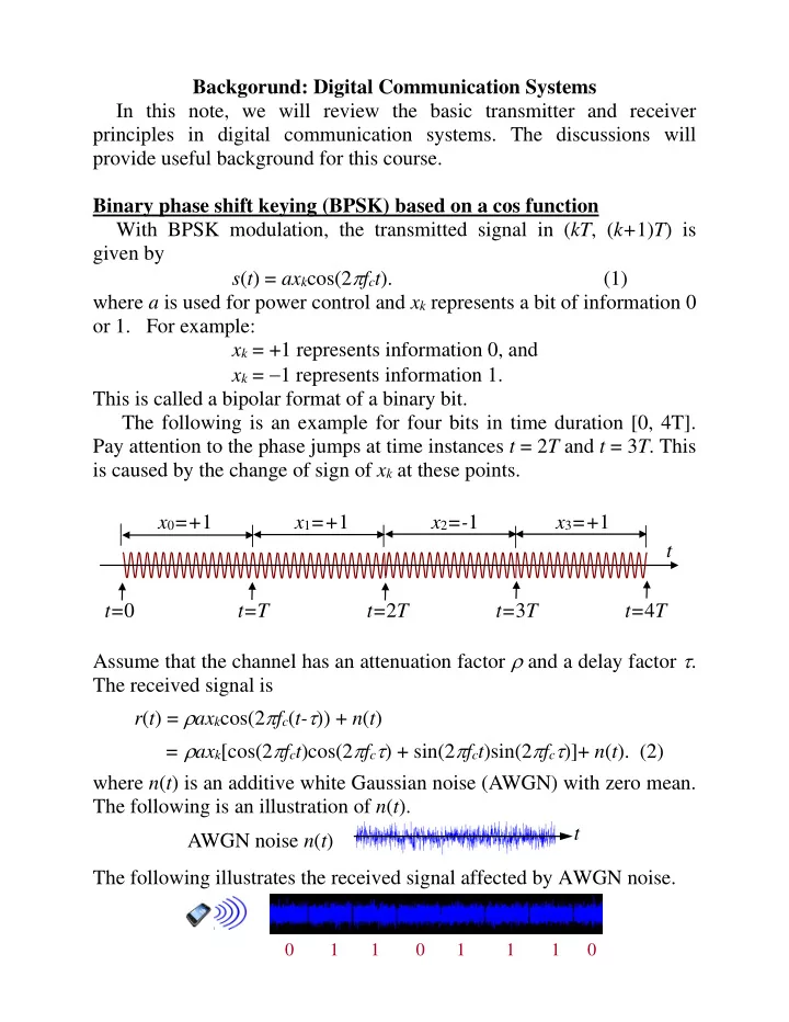
Backgorund: Digital Communication Systems In this note, we will review the basic transmitter and receiver principles in digital communication systems. The discussions will provide useful background for this course. Binary phase shift keying (BPSK) based on a cos function With BPSK modulation, the transmitted signal in (kT, (k+1)T) is given by s(t) = axkcos(2fct). (1) where a is used for power control and xk represents a bit of information 0

• r 1. For example:

xk = +1 represents information 0, and xk = −1 represents information 1. This is called a bipolar format of a binary bit. The following is an example for four bits in time duration [0, 4T]. Pay attention to the phase jumps at time instances t = 2T and t = 3T. This is caused by the change of sign of xk at these points. Assume that the channel has an attenuation factor  and a delay factor . The received signal is r(t) = axkcos(2fc(t-)) + n(t) = axk[cos(2fct)cos(2fc) + sin(2fct)sin(2fc)]+ n(t). (2) where n(t) is an additive white Gaussian noise (AWGN) with zero mean. The following is an illustration of n(t). The following illustrates the received signal affected by AWGN noise. t x0=+1 x1=+1 x2=-1 x3=+1 t=0 t=T t=2T t=3T t=4T AWGN noise n(t) t t

0 1 1 0 1 1 1 0

Some useful equations: The following equations are useful in understading the pricniples of BPSK and QPSK mentioned later. In all cases, we assume that f is very large. In practice, f represents carrier frequency. A typical range of f is 1GHz ~ 5GHZ (i.e., 109 Hz to 5×109 Hz) for the 4G systems.

1 2 cos(2 ) | sin(2 ) sin(2 ) | 2 2

b a

ft dt fb fa f f      = −  



(3a) ( ) ( )

1 2 sin(2 ) | cos(2 ) cos(2 ) | 2 2

b a

ft dt fb fa f f      = − − −  



(3b)

sin(2 )cos(2 ) 0.5 sin(2 2 )

b b a a

ft ft dt ft dt    =  

 

(3c) The following graphic illustration helps to understand the above relationships. Furthermore, we have the following useful approximations:

2

sin (2 ) 0.5 (1 cos(2 2 )) 0.5( )

b b a a

ft dt ft dt b a   = −   −

 

(3d)

2

cos (2 ) 0.5 (1 cos(2 2 )) 0.5( )

b b a a

ft dt ft dt b a   = +   −

 

(3e) Again, the above relationships can be understood using the following graph.

Correlation receiver The following shows a correlation receiver to estimate xk. We repeat (2) as: r(t) = axk[cos(2fct)cos(2fc) + sin(2fct)sin(2fc)]+ n(t). (4) Define

( 1)

( )cos(2 )

k T k c kT

n t f t dt  

+

=  . (5) From (3), we have

( 1) 2

cos (2 ) 0.5

k T c kT

f t dt T 

+





,

( 1) sin(2

)cos(2 )

k T c c kT

f t f t dt  

+





, The output yk in the above receiver can then be expressed as (6) Assume that  is known. We estimate xk using yk and the following rule: (7a) (7b) Note that k is unknown, which may cause detection error. We model k as Gaussian distributed with zero mean and variance = 0.52TN0, where N0 is called single-sided channel noise density. N0 is a measurement of channel noise level. The performance of the above receiver is determined by the following signal to noise ration (SNR)

( )

( )

( )

2 2 2 2 2 2 2

0.5 cos 2 0.5 cos 2 variance of 0.5

c c k

aT f a f T SNR N T        = =

( )( )

2 2

2 cos 2 /

c b

f E N    =

. (8) where Eb=0.5a2T is the transmitted energy per bit (based on (3b)). Note that SNR is affected by Eb, path gain  and delay . xk = +1 if yk has the same sign as

( )

0.5 cos 2

c

aT f   

xk = −1

• therwise.

( )

0.5 cos 2

k k c k

y aTx f     = +

yk s(t) =axkcos(2fct) r(t) = axkcos(2fc(t-)) + n(t)



reference cos(2fct)

channel

( 1) k T kT +



In-phase and quadrature signal components The signal above is modulated by cos(2fct). This is usually referred to as the in-phase component. If sin(2fct) is used for modulation, as discussed below, the related signal is called the quadrature compoenent. If the channel delay  is not zero, then part of the in-phase componenet is turned into a quadrature componenet as (see (2)) axksin(2fct)sin(2fc). Such component is orthogonal to the reference cos(2fct) (see the figure and (3)) since

sin(2 )cos(2 )

b a

ft ft dt   



. The related energy is not utilized, which reduces energy efficiency. Binary phase shift keying (BPSK) based on a sin function We can modulate a signal using a sin function as s(t) = axksin(2fct). (9) The received signal is r(t) = axksin(2fc(t-)) + n(t) = axk[sin(2fct)cos(2fc) − cos(2fct)sin(2fc)]+ n(t). (10) The following shows a correlation receiver to estimate xk. Note that the reference is sin(2fct) now. Define

( 1)

( )sin(2 )

k T k c kT

n t f t dt  

+

=  . (11) We can write the output yk in the above receiver as

( )

0.5 cos 2

k k c k

y aTx f     = +

. (12) We can again estimate xk based on yk. The rule is similar to (7). Again, part of the received signal, i.e., axkcos(2fct)sin(2fc), is not utilized. r(t) = axksin(2fc(t-)) + n(t)



reference sin(2fct)

channel

( 1) k T kT +



s(t) =axksin(2fct) yk

Quadrature phase shift keying (QPSK) We can increase transmission speed as well as energy efficiency using both in-phase and quadrature componenets. This is referred to as quadrature phase shift keying (QPSK). The transmitted signal is

Re Im

( ) cos(2 ) sin(2 )

k c k c

s t ax f t ax f t   = − . (13) The received signal is

( )

( )

( )

( )

Re Im

( ) cos 2 sin 2 ( )

k c k c

r t ax f t ax f t n t       = − − − +

Re Re Im Im

[ cos(2 )cos(2 ) sin(2 )sin(2 )] [ sin(2 )cos(2 ) cos(2 )sin(2 )] ( )

k c c k c c k c c k c c

a x f t f x f t f a x f t f x f t f n t               = + + − + + (14) The following receiver is used for detection. Similar to the discussions earlier, we can shown the following.

( ) ( )

( )

Re Re Im Re

0.5 cos 2 sin 2

k k c k c k

y aT x f x f       = + + , (15a)

( ) ( )

( )

Im Re Im Im

0.5 sin 2 cos 2

k k c k c k

y aT x f x f       = − + + . (15b) Now we introduce notations:

Re Im

=

k k k

x x jx + , (16a)

Re Im

=

k k k

y y jy + , (16b)

( ) ( )

( )

=0.5 cos 2 sin 2

c c

h T f j f      −

, (16c)

Re Im k k k

j    = + . (16d) Then (15) and (16) lead to a very simple expression: (17)

k k k

y ahx  = + ykIm

ykRe r(t)



−sin(2fct)



cos(2fct) quadrature branch in-phase branch

 

Detection for QPSK We can carry out detection using the above graphis illustration. Assume that hk is know. Without noise k, we can find four noiseless possibilities for yk. With noise k, the actual yk is not on these four

• points. We can use the minimum Euclidian distance to find the best
• estimate. For example, for the received signal shown by the “star”

above, the best estimate is the “diamond” since it is closest to the “star”. Notes:

• The transmitted and received signals are all real. The complex

notations are used only for simplicity. We call

Re Im k k k

x x jx = +

a QPSK modulated symbol. It is a simplified notation for the actual signal

Re Im

( ) cos(2 ) sin(2 )

k c k c

s t ax f t ax f t   = − .

• The received signal consists of two parts, i.e.,

Re k

y

and

Im k

y

. They are both real signals. Complex notation is again used only for simplicity.

• Since exp(jz) = cos(z) + jsin(x). We can write h in a phasor form:

( )

=0.5 exp 2 .

c

h T j f    −

Here  is refered to as channel magnitude, ||2 as channel power gain (or simply channel gain) and  as channel delay. Both  and  are determined by channel only. A constant factor 0.5T is introduced by the intergration operation at the receiver.

• In the QPSK receiver, both in-phase and quadrature compoenets can

be fully utilized. Such a structure can also be used to detect a BPSK signal with improved power efficiency.

• 1 +1

+j

• j

Re k

x

Im k

jx ×ah

Im k

jy

Re k

y

received yk with noise four possibilities for yk without noise

The Q-Function In probability theory, the Gaussian distribution is considered the most important probability distribution in statistics. This is why it is also called normal distribution. It means that most things follow this distribution “normally”.

2 2

( ) 2

1 ( ) 2

x m

p x e





− −

=

For example, temperature, water level, incomes, exam results,… Define

2

2

1 ( ) 2

t x

Q x e dt 

 −





Then for a Gaussian distribution,

2 2 2

( ) 2 2 ' ' '

1 1 ' Pr( ') ( ) ( ) 2 2

x m t x m t x m x x

x m x x p x dx e dx e dt Q

  

  

− = − −    − −

−  = = = =

  

• r simply

' Pr( ') ( ) x m x x Q  −  =

Some useful relationships are as follows: Therefore 1-Q(-x) = Q(x) i.e., Q(-x) + Q(x) =1

Error events in a communication system We now consider the impact of noise on detection error in a communication system. We will assume that the noise is Gaussian. Consider the following system model. y = xC + . Here

• x=1 represents a bit of information,
• C is used to adjust transmission power (noting that power = C2),
• h is a Gaussian distributed variable with mean = 0 and variance =

2. The receiver does not know x (otherwise why do we bother to transmit). How can receiver find x? Let us guess x as follows:

• If y>0, we guess that x = 1.
• If y0, we guess that x = -1.

Is this method 100% correct? Of course not. Then what is the error probability? x

transmitted signal for x=-1

Bit error rate (BER) Is the average bit error rate (i.e. BER) 2Q(C/s). No. The probability of x= 1 is 0.5 and the probability of x =-1 is also 0.5. Hence the BER is still Q(C/s).

Bit error rate and SNR From the above discussions,

2 2

BER C C Q Q       = =          

. Here C2/2 is referred to as SNR. Clearly, we can see that BER is a decreasing function of SNR. Summary With QPSK modulation, the signals involved can be expressed using the following concise notations:

( )

Re Im

=

k k k k k

y y jy h ax  + =  +

,

( )

Re Im

= 0.5 exp 2

k k c

h h jh T j f    + = −

,

Re Im

=

k k k

x x jx + ,

Re Im k k k

j    = + . Information is carried in

k

x . The total transmitted power is |a|2 for both real and imaginary parts. (Recall that the average power of cos or sin are both 0.5.) Channel power gain is 2 and channel delay is. For a BPSK system, BER is a decreasing function of SNR, given by

( )

2 2

BER / Q C  =

.