19-11-20 Neutral theory 2 (2019 abridged): Neutral theory of - PDF document

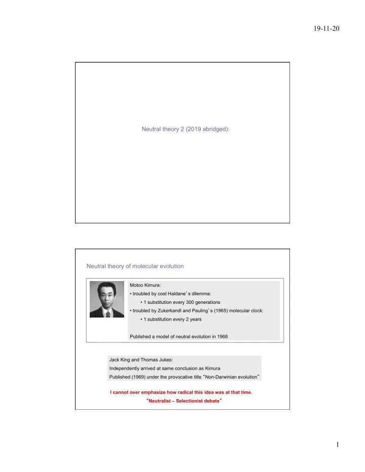
19-11-20 Neutral theory 2 (2019 abridged): Neutral theory of molecular evolution Motoo Kimura: • troubled by cost Haldane ’ s dilemma: • 1 substitution every 300 generations • troubled by Zukerkandl and Pauling ’ s (1965) molecular clock: • 1 substitution every 2 years Published a model of neutral evolution in 1968 Jack King and Thomas Jukes: Independently arrived at same conclusion as Kimura Published (1969) under the provocative title “ Non-Darwinian evolution ” I cannot over emphasize how radical this idea was at that time. “ Neutralist – Selectionist debate ” 1

19-11-20 Neutral theory 1.0 allele frequency A C G 0 T 1. Mutation 2. Polymorphism Neutral theory: connected these is a new (radical) way 3. Substitution neutral theory of molecular evolution (Kimura 1968) k = rate of nucleotide substitution at a site per generation [year] k = new mutations × probability of fixation the number of new mutations 2 N µ v arising in a diploid population the fixation probability of a 12 N v new mutant by drift the substitution (fixation) k = 2 N µ × 1 2 N v rate , k k = µ the elegant simplicity of neutral theory : 2

19-11-20 Neutral theory of molecular evolution Neutral theory: the rate of evolution is independent of effective population size • mutation-drift equilibrium (steady-state between gain and loss) • assumes (i) neutrality and (ii) constant mutation rate • polymorphism is simply a phase of evolution ( mutation, polymorphism and substitution are not separate processes ) k = µ neutral theory: Evolution by natural selection: Kimura 1957 & 1962 • rate depends on mutation rate and population size and intensity of selection • generalization of Wright’s (1938) work 2 s ij prob. of fixation: − 4 Ns ij 1 − e Remember the genetic drift lecture … If we run this simulation long enough it will go to fixation or loss; it just takes much longer • rate to fixation [under drift] slows with increasing in N e • ultimate fate is fixation or loss • Larger N e yield larger residence time of a polymorphism in a population 3

19-11-20 N e = 5000 Generations = 30 Generations = 50 Generations = 500 Generations = 1000 The average time to fixation is 4 N e generations Time to fixation ( t ) of new alleles in populations with different effective sizes. Note that most new mutations are lost from the population due to drift and those mutations are NOT shown. The time to fixation (as an average) is longer in populations with large size. N e = small 1 Allele frequency 0 t N e = large 1 Allele frequency 0 t A slice in time for each population is shown by a dotted vertical line ( ). Note that at such a slice in time the population with larger effective size is more polymorphic as compared with the smaller population. 4

19-11-20 The average time between neutral substitutions is the reciprocal of k ( µ ) µ Mean time between mutation ev ents (1/ 2 N e ) is much shorter in the larger population because number of new mutations is on average = µ × ´ 2Ne (for diploid organisms). The mutation rate ( µ ) is the same in both populations, but numbers differ because of differences in population size (2 N e ). Mutation event N e = small 1 1 2 3 k =3 Allele frequency 0 m ean 1/ µ 2N e µ N = large e 1 1 2 3 k =3 Allele frequency 0 m ean 1/ µ 2 N e µ 2 The population attains an equilibrium substitution rate ( k = µ ) k = µ neutral theory: In words: Large populations: high number of new mutants each generation (2 N e is high) but probability of fixation is low (1/ 2 N e ) Small populations: lower number of new mutants each generation (2 N e is lower), but each has a higher probability of fixation (1/ 2 N e is larger) 5

19-11-20 The average time between neutral substitutions is the reciprocal of k ( µ ) µ Mean time between mutation ev ents (1/ 2 N e ) is much shorter in the larger population because number of new mutations is on average = µ × ´ 2Ne (for diploid organisms). The mutation rate ( µ ) is the same in both populations, but numbers differ because of differences in population size (2 N e ). Mutation event N e = small 1 1 2 3 k =3 Allele frequency 0 m ean 1/ µ 2N e µ “ molecular clock ” N = large e 1 1 2 3 k =3 Allele frequency 0 m ean 1/ µ 2 N e µ 2 Important interpretation: Under neutral theory, the mean rate of evolution is constant over time. This is the so-called “ molecular clock ”. The mean waiting time until a substitution also constant over time. The actual “waiting time” is a random variable because mutation and drift are stochastic. (the clock is “sloppy”) If evolution is in state i , then we wait an exponentially distributed amount of time with a constant mean rate: start observing the process here 3 rd event 1 st event 2 nd event A time waiting time = − 1 λ log e ( u ) 1. λ !=!rate!=! q ii ! 2. u !=!uniform(0,1)!random!number! 6

19-11-20 The average time between neutral substitutions is the reciprocal of k ( µ ) µ Mean time between mutation ev ents (1/ 2 N e ) is much shorter in the larger population because number of new mutations is on average = µ × ´ 2Ne (for diploid organisms). The mutation rate ( µ ) is the same in both populations, but numbers differ because of differences in population size (2 N e ). Mutation event N e = small 1 1 2 3 k =3 Allele frequency 0 m ean 1/ µ µ 2N e N = large e 1 1 2 3 k =3 Allele frequency 0 m ean 1/ µ 2 N e µ 2 It looks like there is more variability within the population when Ne is large The population attains an equilibrium ( steady-state ) polymorphism H e = 4 N e µ / (1+ 4 N e µ ) this result assumes an “ infinite alleles model ” θ = 4 N e µ population geneticists are obsessed with the µ parameter 7

19-11-20 The population attains an equilibrium polymorphism Expected equilibrium levels of heterozygosity at a locus as a function of the parameter θ . Heterozygosity will be higher in larger populations. 1 0.9 0.8 0.7 Heterozygosity (H) 0.6 0.5 0.4 0.3 0.2 0.1 0 0 2 4 6 8 10 θ H: Substantial “standing polymorphism” with NO LOAD1 The population attains an equilibrium polymorphism Expected equilibrium levels of heterozygosity at a locus as a function of the parameter θ . Heterozygosity will be higher in larger populations. H: Steady-state 1 0.9 heterozygosity that 0.8 results when increase 0.7 Heterozygosity (H) in alleles due to 0.6 0.5 mutation is exactly 0.4 balanced by their loss 0.3 due to drift. 0.2 0.1 0 0 2 4 6 8 10 θ 8

19-11-20 The average time between neutral substitutions is the reciprocal of k ( µ ) µ Mean time between mutation ev ents (1/ 2 N e ) is much shorter in the larger population because number of new mutations is on average = µ × ´ 2Ne (for diploid organisms). The mutation rate ( µ ) is the same in both populations, but numbers differ because of differences in population size (2 N e ). Mutation event N e = small 1 1 2 3 k =3 Allele frequency 0 m ean 1/ µ µ 2N e N = large e 1 1 2 3 k =3 Allele frequency 0 m ean 1/ µ 2 N e µ 2 we “see” how there could be a difference in steady state heterozygosity when Ne is large vs small Neutral theory of molecular evolution 1. We can compute expectations for long-term mutation + drift equilibrium 2. The standing level of polymorphism is dependent on effective population size 3. The rate of evolution is independent of effective population size (constant, on ave.) 9