10. Repetition Binary Search Trees and Disadvantages of hashing: - PowerPoint PPT Presentation

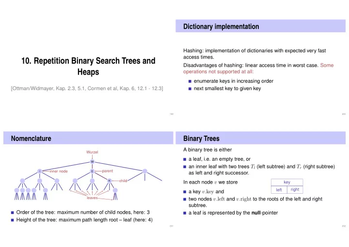
Dictionary implementation Hashing: implementation of dictionaries with expected very fast access times. 10. Repetition Binary Search Trees and Disadvantages of hashing: linear access time in worst case. Some Heaps operations not supported at all: enumerate keys in increasing order [Ottman/Widmayer, Kap. 2.3, 5.1, Cormen et al, Kap. 6, 12.1 - 12.3] next smallest key to given key 199 200 Nomenclature Binary Trees A binary tree is either Wurzel a leaf, i.e. an empty tree, or W an inner leaf with two trees T l (left subtree) and T r (right subtree) parent inner node I E as left and right successor. child K In each node v we store key right left a key v. key and leaves two nodes v. left and v. right to the roots of the left and right subtree. Order of the tree: maximum number of child nodes, here: 3 a leaf is represented by the null -pointer Height of the tree: maximum path length root – leaf (here: 4) 201 202

Baumknoten in Java Baumknoten in Python SearchNode SearchNode public class SearchNode { key (type int ) 5 key 5 int key; SearchNode left; class SearchNode: SearchNode right; def __init__(self, k, l=None, r=None): self.key = k 3 8 3 8 SearchNode(int k){ self.left, self.right = l, r key = k; self.flagged = False left = right = null; null null null None None None } 2 2 } left (type SearchNode ) right (type SearchNode ) left right null null None None 203 204 Binary search tree Searching A binary search tree is a binary tree that fulfils the search tree Input: Binary search tree with root r , key k property : Output: Node v with v. key = k or null Every node v stores a key 8 v ← r Keys in left subtree v.left are smaller than v.key while v � = null do 4 13 if k = v. key then Keys in right subtree v.right are greater than v.key return v else if k < v. key then 10 19 16 v ← v. left else 9 7 18 v ← v. right Search (12) → null return null 5 10 17 30 2 9 15 99 205 206

Insertion of a key Remove node Insertion of the key k 8 Three cases possible: 8 Search for k Node has no children 4 13 If successful search: output 3 13 Node has one child error 5 10 19 5 10 19 Node has two children No success: replace the 9 reached leaf by a new node [Leaves do not count here] 4 9 Insert (5) with key 207 208 Remove node Remove node Node has no children Node has one child Simple case: replace node by leaf. Also simple: replace node by single child. 8 8 8 8 3 13 3 13 3 13 5 13 remove (4) remove (3) − → − → 5 5 5 10 19 10 19 10 19 4 10 19 4 9 9 4 9 9 209 210

Remove node By symmetry... Node has two children The following observation helps: the 8 8 smallest key in the right subtree v.right Node has two children 3 13 (the symmetric successor of v ) 3 13 Also possible: replace v by its symmetric is smaller than all keys in v.right 5 10 19 predecessor. 5 10 19 is greater than all keys in v.left 4 9 and cannot have a left child. 4 9 Solution: replace v by its symmetric suc- cessor. 211 212 Algorithm SymmetricSuccessor( v ) Traversal possibilities preorder: v , then T left ( v ) , then Input: Node v of a binary search tree. T right ( v ) . Output: Symmetric successor of v 8 8, 3, 5, 4, 13, 10, 9, 19 w ← v. right x ← w. left 3 13 postorder: T left ( v ) , then T right ( v ) , then while x � = null do v . w ← x 5 10 19 4, 5, 3, 9, 10, 19, 13, 8 x ← x. left inorder: T left ( v ) , then v , then T right ( v ) . 4 9 return w 3, 4, 5, 8, 9, 10, 13, 19 213 214

Height of a tree Analysis The height h ( T ) of a tree T with root r is given by � Search, Insertion and Deletion of an element v from a tree T 0 if r = null h ( r ) = requires O ( h ( T )) fundamental steps in the worst case. 1 + max { h ( r. left) , h ( r. right) } otherwise. The worst case run time of the search is thus O ( h ( T )) 215 216 Possible Heights Further supported operations Min( T ): Read-out minimal value in 1 The maximal height h n of a tree with n inner nodes is given with O ( h ) 8 h 1 = 1 and h n +1 ≤ 1 + h n by h n ≥ n . ExtractMin( T ): Read-out and remove 2 The minimal height h n of an (ideally balanced) tree with n inner minimal value in O ( h ) 3 13 i =0 2 i = 2 h − 1 . nodes fulfils n ≤ � h − 1 List( T ): Output the sorted list of 5 10 19 elements Thus Join( T 1 , T 2 ): Merge two trees with ⌈ log 2 ( n + 1) ⌉ ≤ h ≤ n 4 9 max( T 1 ) < min( T 2 ) in O ( n ) . 217 218

Degenerated search trees [Probabilistically] 4 19 5 13 A search tree constructed from a random sequence of numbers 9 provides an an expected path length of O (log n ) . 8 10 Attention: this only holds for insertions. If the tree is constructed by 5 13 9 9 random insertions and deletions, the expected path length is O ( √ n ) . 10 8 4 8 10 19 Balanced trees make sure (e.g. with rotations ) during insertion or 13 5 Insert 9,5,13,4,8,10,19 deletion that the tree stays balanced and provide a O (log n ) ideally balanced Worst-case guarantee. 19 4 Insert 4,5,8,9,10,13,19 Insert 19,13,10,9,8,5,4 linear list linear list (not shown in class) 220 219 [Max-]Heap 8 Heap and Array Binary tree with the following prop- Tree → Array: erties 22 root children ( i ) = { 2 i, 2 i + 1 } 1 complete up to the lowest [1] parent ( i ) = ⌊ i/ 2 ⌋ 20 18 level 22 [2] [3] parent 2 Gaps (if any) of the tree in 16 12 15 17 parent 20 18 the last level to the right [4] [5] [6] [7] 20 18 16 15 3 8 22 12 17 2 11 14 3 2 8 11 14 3 Heap-Condition: child 16 12 15 17 1 2 3 4 5 6 7 8 9 10 11 12 [8] [9] [10] [11] [12] Max-(Min-)Heap: key of a Children 3 8 2 11 14 child smaller (greater) that Depends on the starting index 9 that of the parent node 8 Heap(data structure), not: as in “heap and stack” (memory allocation) 9 For array that start at 0 : { 2 i, 2 i + 1 } → { 2 i + 1 , 2 i + 2 } , ⌊ i/ 2 ⌋ → ⌊ ( i − 1) / 2 ⌋ 221 222

Height of a Heap Insert A complete binary tree with height 10 h provides 22 h − 1 20 18 � 1 + 2 + 4 + 8 + ... + 2 h − 1 = 2 i = 2 h − 1 Insert new element at the first free 16 12 15 17 position. Potentially violates the heap i =0 property. 3 2 8 11 14 nodes. Thus for a heap with height h : Reestablish heap property: climb 22 2 h − 1 − 1 < n ≤ 2 h − 1 successively 20 21 Worst case number of operations: 2 h − 1 < n + 1 ≤ 2 h ⇔ O (log n ) 16 18 12 17 Particularly h ( n ) = ⌈ log 2 ( n + 1) ⌉ and h ( n ) ∈ Θ(log n ) . 3 2 8 11 14 15 10 here: number of edges from the root to a leaf 223 224 Algorithm SiftDown( A, i, m ) Remove the maximum 21 Input : Array A with heap structure for the children of i . Last element m . 20 18 Output : Array A with heap structure for i with last element m . Replace the maximum by the lower while 2 i ≤ m do right element 16 12 15 17 j ← 2 i ; // j left child Reestablish heap property: sift down if j < m and A [ j ] < A [ j + 1] then 3 2 8 11 14 j ← j + 1 ; // j right child with greater key successively (in the direction of the 20 if A [ i ] < A [ j ] then greater child) swap( A [ i ] , A [ j ] ) Worst case number of operations: 16 18 i ← j ; // keep sinking down O (log n ) else 14 12 15 17 i ← m ; // sift down finished 3 2 8 11 225 226

Sort heap Heap creation 5 7 6 4 1 2 2 6 4 5 1 7 swap ⇒ 6 5 7 ⇒ 4 2 1 siftDown A [1 , ..., n ] is a Heap. Observation: Every leaf of a heap is trivially a correct heap. 1 5 4 2 6 7 swap ⇒ While n > 1 5 4 2 1 6 7 ⇒ siftDown swap( A [1] , A [ n ] ) 5 ⇒ 1 4 2 6 7 swap Consequence: Induction from below! SiftDown( A, 1 , n − 1 ); 4 1 2 5 6 7 siftDown ⇒ n ← n − 1 5 6 7 ⇒ 2 1 4 swap 2 1 4 5 6 7 siftDown ⇒ 1 2 4 5 6 7 ⇒ swap 227 228 Algorithm HeapSort( A, n ) Analysis: sorting a heap Input : Array A with length n . Output : A sorted. // Build the heap. SiftDown traverses at most log n nodes. For each node 2 key for i ← n/ 2 downto 1 do comparisons. ⇒ sorting a heap costs in the worst case 2 log n SiftDown( A, i, n ); comparisons. // Now A is a heap. for i ← n downto 2 do Number of memory movements of sorting a heap also O ( n log n ) . swap( A [1] , A [ i ] ) SiftDown( A, 1 , i − 1 ) // Now A is sorted. 229 230