1 The Balassa-Samuelson effect in central Europe: a disaggregated - - PDF document

SLIDE 1

The Balassa-Samuelson effect in central Europe: a disaggregated analysis

1

Dubravko Mihaljek Bank for International Settlements CH-4002 Basel, Switzerland

E-mail: Dubravko.Mihaljek@bis.org

Paper presented at the conference Exchange rate strategies during the EU enlargement Budapest, 27–30 November 2002 Current version: 8 November 2002 First draft: 24 June 2002

1

The views expressed are those of the author and do not necessarily represent those of the Bank for International

• Settlements. I would like to thank Marc Klau for expert research assistance, and Palle Andersen, Balász Égert,

Christoph Fischer, Boštjan Jazbec, Velimir Šonje and participants of the 8th Dubrovnik Economic Conference for helpful comments.

SLIDE 2

2

Dubravko Mihaljek

The Balassa-Samuelson effect in central Europe: a disaggregated analysis Summary

This paper aims to explain inflation differentials observed over the past decade between six central European economies – Croatia, the Czech Republic, Hungary, Poland, Slovakia and Slovenia – and the euro area in terms of differential productivity growth. The coverage of tradable and non-tradable industries is broader and more detailed than in previous studies and the data samples are larger, as quarterly data for up to ten years are used. The main conclusion is that differential productivity growth – ie, the Balassa-Samuelson effect – does not seem to have played a major role in determining either inflation differentials vis-à-vis the euro area, or

• verall CPI inflation in central European countries. The paper shows that one needs to distinguish carefully

between empirical evidence that faster productivity growth in tradable industries contributes to rising relative prices of non-tradables, and evidence that productivity differentials contribute to inflation differentials between central European economies and the euro area. Although relative prices of non- tradables in central Europe are rising more or less in line with relative productivity of tradables, the same phenomenon has been observed in the euro area. As a result, productivity differentials vis-à-vis the euro area explain on average only between 0.2 and 2 percentage points of annual inflation differentials between central European countries and the euro area. Moreover, productivity differentials between tradable and non-tradable industries in general explain only a small proportion of domestic inflation in central European

• countries. Earlier studies that estimated this “domestic” Balassa-Samuelson effect to be larger have often

neglected productivity growth in non-tradable sectors, which has been quite high in many countries. These results have important policy implications. If EU accession countries find it difficult to satisfy the Maastricht inflation criterion, they will probably have to look for reasons beyond differential productivity growth, at least based on the performance of their tradable and non-tradable industries to date. Keywords: Balassa-Samuelson effect; Productivity; EU accession; Inflation; Transition.

SLIDE 3

3

Introduction Recent academic and policy discussions about monetary and exchange rate policies in EU accession countries have noted a possible conflict between a significant trend appreciation of real exchange rates in these countries and the inflation and exchange rate criteria for EMU membership (see eg Szapáry, 2000). If the productivity growth differential between the traded and non-traded goods sectors is larger in the accession countries than in euro area on account of faster productivity catch-up in the traded goods sector than in the non-traded sector, the relative price of non-traded goods to traded goods will be rising faster in the accession country than in the euro area. At a given exchange rate, the overall inflation can thus be expected to be higher in the accession countries than in the euro area. To prevent this Balassa-Samuelson effect from manifesting itself and to produce an inflation rate below the Maastricht ceiling, monetary policy may have to be kept very tight, which could result in a growth slowdown. If the accession countries return to full employment following EMU membership, the inflation rate would, however, continue to exceed that

• f the older EMU members by the margin implied by the Balassa-Samuelson effect, for as long as these

intersectoral productivity growth differentials have not converged (Buiter and Grafe, 2002). These observations imply a dilemma for monetary policies pursued by EU accession countries with fixed exchange rates. The dilemma is less pronounced for those EU accession candidates whose exchange rates are floating: the Czech Republic, Hungary, Poland and Slovakia. If monetary policy in these countries were to keep inflation below the Maastricht ceiling but the inflation differential warranted by the Balassa- Samuelson effect was greater than the 1½ percentage point margin (at a given exchange rate and at full capacity), the equilibrium response of the nominal exchange rate would be to appreciate (Buiter and Grafe, 2002). The Balassa-Samuelson effect would have to be very large to exhaust the 15% bands of the ERM in two years, assuming that exchange rate starts in the middle of the band. However, a floating rate regime has drawbacks of its own, so these countries would not necessarily find it easier to join the EMU. The available estimates of the Balassa-Samuelson effect in the transition economies range from zero to 4 percentage points per annum (see Table 1). However, most of these studies do not test the extent to which inflation differences between accession countries and the euro area can be explained by productivity

• differentials. Rather, they test a related hypothesis developed by Baumol and Bowen (1966) that prices of

services grow faster than those of manufactured goods due to faster productivity growth in manufacturing

• industries. This effect in itself is not sufficient to lead to a rise in the general price level – prices of

manufactured goods have tended to fall in many countries in recent years as a result of increased domestic and foreign competition. Moreover, the mere presence of faster productivity growth in manufacturing is not sufficient to “justify” a rate of inflation in the transition economies that is higher than in the EU. The inflation differential between countries can be explained in terms of underlying productivity developments only if the productivity growth differential (between traded and non-traded industries) is higher in accession countries than in the euro area. Against this background, this paper aims at assessing, with some degree of accuracy, the empirical significance of the Balassa-Samuelson effect in six central European economies – Croatia, the Czech Republic, Hungary, Poland, Slovakia and Slovenia. The main conclusion is that, despite evidence of higher productivity growth, productivity differentials in central Europe explain only a small proportion of inflation differentials vis-à-vis the euro area. The next two sections lay out the analytical and empirical framework used in the paper. The remaining sections compare data on productivity growth in tradable and non- tradable industries, attempt to account for inflation differentials in terms of differential productivity growth, and provide preliminary estimates of the Balassa-Samuelson effect. Analytical framework Balassa (1964) and Samuelson (1964) identified productivity growth differentials between the sectors producing tradable and non-tradable goods as a factor introducing systematic biases into the relationship between exchange rates and relative prices. Historically, productivity growth in the traded goods sector has been faster than in the non-traded goods sector. By the law of one price, the prices of tradables tend to get equalised across countries, while the prices of non-tradables do not. Higher productivity in the tradable goods sector will bid up wages in that sector and, with labour being mobile, wages in the entire economy will rise. Producers of non-tradables will be able to pay the higher wages only if the relative price on non- tradables rises. This will in general lead to an increase in the overall price level in the economy.

2 2

Another consequence, which was the real focus of Balassa and Samuelson, is that the prices of a common basket of goods in two countries measured in a common currency will differ systematically in the presence of long-run productivity differentials.

SLIDE 4

4

To formalise this model, the aggregate price level is first decomposed into its traded and non-traded components, both at home and abroad: pt = αpt

T + (1 – α)pt NT

(1) pt

* = α*pt T* + (1 – α*)pt NT*

(1') where pt

T denotes the price of traded goods, pt NT denotes the price of non-traded goods, and α denotes the

share of traded goods in each economy. The real exchange rate q is defined as the relative price of goods produced abroad (measured in domestic currency) to domestically produced goods:

t t t t

p p e q − + = ) (

*

(2) where et is the nominal exchange rate expressed in units of the domestic currency per unit of the foreign

• currency. Substituting (1) and (1') in (2) and expressing the result in terms of the differences, the following

expression can be obtained: )] )( 1 ( ) )( 1 [( ) (

* * * * T t NT t t T t NT t T t T t t t

p p p p p p e q ∆ − ∆ − − ∆ − ∆ − + ∆ − ∆ + ∆ = ∆ α α (3) If the law of one price holds in the tradable sector, then: ∆pT = ∆e + ∆pT* (4) ie, the first term on the right hand side of (3) will be zero. Next, an expression for the movements of relative prices in terms of the productivity differentials between traded and non-traded goods is derived. A model of a small open economy with the following sectoral production functions is assumed (time subscripts are omitted to simplify notation and since it is assumed that there are no adjustment costs):

γ γ −

=

1

) ( ) (

T T T T

K L A Y

(5)

δ δ −

=

1

) ( ) (

NT NT NT NT

K L A Y

(5') where Y denotes output of traded and non-traded goods; and A, K, and L are productivity, capital and labour inputs. Assuming perfect mobility of capital both internationally and across the two sectors internally, as well as perfect competition in both sectors, profit maximisation implies:

γ

γ

−

• −

=

T T T

L K A R ) 1 (

(6)

δ

δ

−

• −

=

NT NT NT NT

L K A P R ) 1 (

(7)

γ

γ

−

• =

1 T T T

L K A W

(8)

δ

δ

−

• =

1 NT NT NT NT

L K A P W

(9) where R is the rental rate on capital (determined in world markets), W is the wage rate (measured in tradables) and PN is the relative price of non-tradables. A key insight of Balassa and Samuelson is that with perfect capital mobility, the relative price of non- tradables PN is governed entirely by the production side of the economy. Equations (6)–(9) involve four equations in four variables, KT/LT, KNT/LNT, W and PNT, which can be solved recursively.

3 3

Given the constant returns to scale production functions, equation (6) implies a unique level of KT/LT consistent with the world rate of return on capital R. Given KT/LT, equation (8) determines the economy-wide wage rate W. The remaining two equations then determine KNT/LNT and PNT.

SLIDE 5

5

By log-differentiating equations (6)–(9), one can obtain the following (domestic) version of the Balassa- Samuelson hypothesis:

NT T T NT

a a c p p p −

• +

= − = γ δ (10) where lower-case letters denote logarithms, c is a constant term that includes the real interest rate and factor intensities (which are taken as given), and aT and aNT are productivity growth rates in the two

• sectors. One important point, which is generally overlooked in the literature and empirical work, is that if

non-traded goods are more labour intensive (ie, δ > γ), then even a balanced growth of productivity (aT = aNT) will lead to an appreciation of the relative price of traded goods.

4 The percentage change in the relative

price of traded goods will be equal to the productivity growth differential only if both sectors have the same degree of labour intensity. Another implication of equation (10) is that in the small open economy with perfect labour mobility, demand factors do not affect the relative price of non-tradables, they only affect a country's consumption basket. However, if capital is not fully mobile or the economy is large, R is no longer tied down by world markets. In this case, equations (6)–(9) have to be supplemented by the demand side of the model. Substituting (10) into (3) and using definitions (2) and (4) one obtains:

] )[ 1 ( ] )[ 1 (

* * * * * * NT t T t t NT t T t t t t t

a a a a e p p ∆ − ∆

• −

− ∆ − ∆

• −

+ ∆ = ∆ − ∆ γ δ α γ δ α

(11) The difference between the rates of inflation in an accession country and the euro area can thus be expressed as a sum of the nominal exchange rate depreciation of the accession country’s currency vis-à- vis the euro, ∆e, and a weighted average of the productivity growth differentials between the traded and non-traded goods sectors in the accession country ( ∆ aT – ∆ aNT) and the euro area ( ∆ aT

* – ∆ aNT *).

5

A final analytical point to note is that the Balassa-Samuelson effect is closely related to – but distinct from – the so-called Baumol-Bowen effect. Baumol and Bowen (1966) argued that within a country there is a broad tendency for the prices of service intensive goods (education, health care, auto repair, banking, etc.) to rise over time as, historically, productivity growth in these activities has tended to be much slower than in the more capital intensive manufacturing industries. Although there is a considerable overlap between non- tradables and service-intensive goods, the presence of a rising relative price of services, established on the basis of equation (10) or its equivalent, is not necessarily sufficient to imply a Balassa-Samuelson

• effect. As noted above, a higher rate of inflation at home than abroad can be explained as an equilibrium

phenomenon only if differential productivity growth between the sectors producing traded and non-traded goods is greater at home than abroad. Empirical framework Most studies investigating the Balassa-Samuelson effect in transition economies use as the dependent variable a measure of the relative price of non-tradables and estimate a version of equation (10) (see Table 1).

6 In fact, these studies estimate the Baumol-Bowen effect, so even when they establish a strong positive

correlation between differential productivity growth and the relative price of non-tradables, this does not show that higher inflation in the accession countries relative to the euro area can be justified as an equilibrium phenomenon.

4

This point is emphasised by Froot and Rogoff (1995).

5

An equivalent expression can be derived within the Scandinavian model of inflation (Aukrust, 1977), which explains the domestic rate of inflation (π) and the increases in domestic money wages in the open (or “exposed”) and “sheltered” sectors through an exogenously given rate of increase in the foreign price level, π*, and the development of labour productivity in the two sectors (aE and aS): π = π* + αS(aE – aS).

6

This is also true of many studies of the Balassa-Samuelson effect in other countries, eg, De Gregorio, Giovannini and Wolf (1994) and Swagel (1999). One exception is Alberola-Ila and Tyrväinen (1998).

SLIDE 6

6

The remaining studies focus on the evolution of real effective exchange rates (REER).

7 One problem with

this approach is that multilateral REER indices are based on constant weights, the use of which is inappropriate given that trade patterns have shifted significantly throughout the transition. Another problem is that REER indices include inflation differentials as well as nominal exchange rate changes vis-à-vis countries outside the euro area. As a result, this approach may lead to inaccurate measurement of the Balassa-Samuelson effect.

8

Only few studies so far have attempted to estimate to what extent inflation differentials between transition economies and the EU can be explained by relative productivity differentials.

9 In particular, equation (11)

has not been tested empirically, even though the policy interest in the Balassa-Samuelson effect is precisely the contribution of differential productivity growth to inflation differentials between EU accession countries and the euro area. This paper will attempt to fill this gap. All empirical studies of the Balassa-Samuelson effect – including the present one – also suffer to varying degrees from data measurement problems. First, most studies use annual data for the 1990s and try to compensate for the short time series by pooling data from different transition economies. Such cross- country panels often include very heterogeneous economies, from advanced EU accession candidates in central Europe, to relatively under-developed central Asian CIS economies.

10

Second, the sectoral data used are highly aggregated. The traded goods sector typically includes industry – usually only manufacturing, but often also construction as well as electricity, gas and water supply, industries whose output is only to a small extent traded. The non-traded sector is in some studies the residual (ie, GDP less industry) (see Table 1). In others, it covers all services irrespective of their traded

• content. Some studies do not even consider non-tradables, assuming that productivity growth in the sector

is zero or equal across countries.

11 Another frequent problem is the use of industrial production indices,

which measure gross output rather than value-added, in constructing labour productivity measures. Some additional simplifying assumptions are worth noting. The shares of non-traded goods (1 – α) are typically assumed to be the same across countries. Finally, none of the studies (including this one) considers the case of different relative factor intensities in non-traded and traded sectors (δ/γ).

12 As argued

below, the use of these assumptions in empirical work can significantly affect the size of estimated Balassa-Samuelson effect. In particular, productivity growth in non-tradable industries differs substantially across transition economies as well as between the euro area and these economies. To overcome some of these shortcomings and obtain more reliable empirical estimates, this paper focuses

• n the “full” specification of the Balassa-Samuelson hypothesis and uses a disaggregated analysis:
• The main goal of the paper is to see to what extent inflation differentials between EU accession

candidates and euro area economies can be explained by productivity growth differentials. As argued above, this is one of the key issues for monetary and exchange rate policies in the run-up to EU accession and participation of central European economies in EMU. To address this issue empirically, it is important to look at the “full” version of the of the Balassa-Samuelson hypothesis, ie, equation (11).

7

In a two-country model, the CPI-based real effective exchange rate corresponds to the real exchange rate in equation (2), which was used to derive the Balassa-Samuelson equation (11). Let pT and pN be traded goods price inflation at home, pT* and pN* abroad, and e the rate of nominal exchange rate depreciation, so that pT = e + pT*. Then the evolution of the real exchange rate is: e – [αpT + (1 – α) pN] + [αpT* + (1 – α) pN*], where α is the share of traded goods in consumption, assumed to be same at home and

• abroad. The real exchange rate then changes as: - (1 - α) [(pN - pT) – (pN* - pT*)], ie it appreciates when pN - pT > pN* - pT*.

8

Fischer (2002) points out that, in a model with investment demand, rising productivity in the export sector (which usually requires relatively large capital input and relatively small labour input) raises the equilibrium capital stock and thus investment demand, which in turn increases prices and, ceteris paribus, leads to real exchange rate appreciation. The estimated total effect of productivity on the real exchange rate may thus include not only the pure Balassa-Samuelson effect, but also the investment demand effect.

9

Egert (2002a and 2002b) and Egert et al. (2002) estimate the inflation differential vis-à-vis Germany as a proxy for EU.

10

See eg Coricelli and Jazbec (2001), De Broeck and Sløk (2001), and Jazbec (2001).

11

See Egert (2002a and 2002b).

12

Under the assumptions of same productivity growth in domestic and foreign non-tradable industries, same shares of non-tradables, and same factor intensities, equation (11) simplifies to: ) )( 1 (

* * T t T t t t t t

a a e p p ∆ − ∆ − = ∆ − ∆ − ∆ α . The left-hand side of this equation is then represented in empirical work by the CPI-based real effective exchange rate.

SLIDE 7

7

• The coverage of traded and non-traded industries in this paper is broader and more detailed than in

previous studies. In particular, the traded sector includes not only manufacturing, but also mining, transportation and communications, and tourism, while the non-traded sector includes energy, construction, wholesale and retail trade, real estate and business services, education, health, and personal services (see Appendix);

• The data samples are larger, as quarterly data for up to ten years are used. This makes it possible to

estimate the Balassa-Samuelson effect for individual countries rather than a panel of economies with different structural characteristics. The data series are still very short, however, and are of poor quality for some countries. This highlights the need to interpret the results of analysis cautiously. The empirical analysis proceeds in three steps. First, a preliminary look at the data is taken. Second, inflation differentials between central European economies and the euro area are decomposed on the basis of equation (11), which provides a theoretical model of the long-run relationship between inflation and productivity differentials under given – admittedly, highly restrictive – assumptions.

13 Third, an empirical

counterpart of equation (11) is estimated using standard regression tools. Preliminary look at the data In order to get an impression of the Balassa-Samuelson hypothesis, the sectoral data on productivity and prices in various countries are considered in Charts 1–4. To illustrate the data problem for some countries, most of the series are shown as unadjusted four-quarter percentage changes; in the econometric work, the “dented” series are smoothed using seasonal adjustment or a Hodrick-Prescott filter. The first point to note is that, over the whole sample period, productivity in the traded goods sector has grown faster than in the non-tradable sector, as the first panel for each country shows. The exception is Slovakia, where the growth rate of labour productivity in non-traded industries was higher during 1996–97. According to the theoretical model, faster productivity growth in tradable industries should have implied faster growth of non-traded goods prices. The second panel for each country shows that this has in general been the case. One exception is again Slovakia in the mid-1990s; another is Slovenia in the early 1990s. The core of the productivity hypothesis is shown in the third panel for each country. Relative prices of non- tradables have tended to rise as relative productivity in the tradable sector has increased. This provides indication of the Baumol-Bowen effect. From Chart 4 it can be noted, however, that productivity growth differential in the euro area had also been large. Thus, despite indications that relative prices of non- tradables in central European countries increased in line with relative productivity of tradables, one should not jump to the conclusion that the Balassa-Samuelson effect is present vis-à-vis the euro area. The data also suggest that the assumption of the Balassa-Samuelson model on uniform wage growth – due to sectoral labour mobility – seems to hold in most countries (see fourth panel for each country in Charts 1–4). However, the growth rate of wages in Croatia’s non-tradable industries has been consistently higher, despite higher labour productivity growth in traded goods industries. The same phenomenon could be observed in Slovakia as well as the Czech Republic (in 2000) and in Poland (in 1999). In the latter two cases, however, the deviations probably reflect measurement problems. Non-uniform growth of wages suggests that relative wages may have played an additional role in the long-run relationship between sectoral prices and productivity growth differentials in Croatia and Slovakia. Relative wages were therefore used as an additional explanatory variable in deriving the Balassa-Samuelson effect in these two countries.

13

As noted above, if purchasing power parity does not hold for tradable goods or capital is not fully mobile, demand side factors will also have a role in determining the inflation differentials.

SLIDE 8

Table 1. Selected empirical studies of the Balassa-Samuelson effect in central and eastern European economies Sectoral decomposition Study author(s) Country sample Dependent variable Tradables Non-tradables Other explanatory variables Estimation method Estimate of the Balassa- Samuelson effect

(percentage points per annum)

Simon and Kovács (1998) Hungary, 1991–96 REER Manufacturing (excl. agriculture, mining and energy) Services (excl. public administration) — No regressions 2.9 Cipriani (2000) 10 accession candidates, 1995–99, quarterly data PN/PT (NT/T goods and services from CPI) Industry and mining (goods from CPI) Residual (excl. agriculture) (services from CPI) — OLS 0.5–0.7 Rother (2000) Slovenia, 1993–98, quarterly data PN/PT (producer price index/labour costs) Manufacturing Residual (excl. agriculture) Monetary base, budget deficit/GDP, gvt cons/GDP OLS 1–4 De Broeck and Sløk (2001) 25 transition economies, 1993–98 REER Industry and construction Services Agricultural productivity, broad money, openness, budget balance, terms of trade, commodity prices Pooled mean group estimation 0.2–0.6 Egert (2002a) 12 transition economies, 1993–2001, quarterly data PN/PT (CPI/PPI) RER (D-mark) Industry Not considered (productivity set at zero) — VAR and panel cointegration 0.9 (pooled estimates) 0–3.5 (individual country estimates) Fischer (2002) 10 accession candidates, 1993–99 REER Industry Services Agricultural productivity, gvt cons/GDP, world real interest rate, terms of trade, commodity prices SUR fixed effects 0.7–2.2 (Partly attributed to investment demand channel) Halpern and Wyplosz (2001) 8 accession candidates, Russia, 1991–98 PN/PT (services/non- food manufactured goods from CPI) Industry Services GDP/capita, inflation acceleration term, lagged relative price GLS 3 Coricelli and Jazbec (2001) 19 transition economies, 1990–98 PT/PN (sectoral GDP deflators) Manufacturing, mining, energy, construction Residual Share of non-tradables consumption, government consumption, “structural misalignment” measure Fixed effects panel estimation 0.9–1.2 Arratibel et al (2002) 10 accession candidates, 1990–2001 PN/PT (CPI decomposition

• f NT/T goods and

services) Manufacturing Not considered

• Exch. rate regime, budget

deficit, GDP/capita, wage growth, unemployment, oil price, terms of trade, etc. Method of moments Insignificant

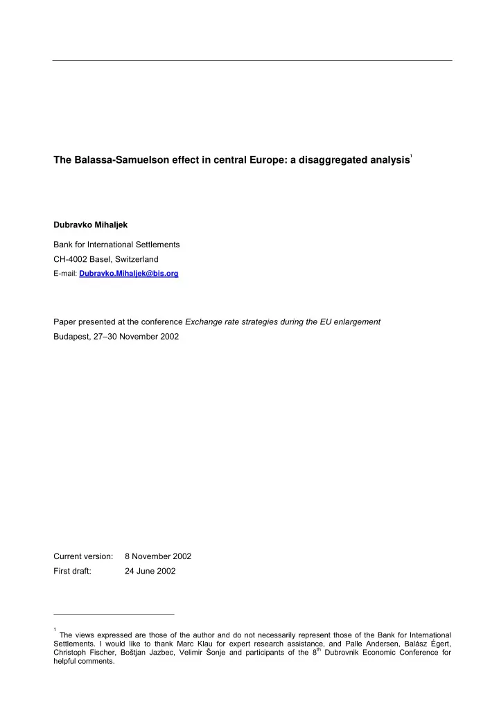
SLIDE 9

Chart 1. Croatia and Slovenia1

1 Dotted lines represent linear time trends. Estimated regression lines show time trend ("x") regressed on the dependent variable ("y") shown in

the legend on the left. HR Labour productivity y = 1.63x + 99.36 y = 0.57x + 103.11 95 105 115 125 135 145 155

1995-1 1995-3 1996-1 1996-3 1997-1 1997-3 1998-1 1998-3 1999-1 1999-3 2000-1 2000-3 2001-1 2001-3

LPRODT LPRODNT HR Relative productivity T/NT and relative price NT/T y = 0.92x + 96.98 y = 0.70x + 98.33 90 95 100 105 110 115 120 125 130

1995-1 1995-3 1996-1 1996-3 1997-1 1997-3 1998-1 1998-3 1999-1 1999-3 2000-1 2000-3 2001-1 2001-3

RELPROD T/NT RELPRICE NT/T

HR CPI decomposition y = 1.03x + 93.61 y = 2.42x + 95.72 80 90 100 110 120 130 140 150 160 170 180

1994-1 1994-3 1995-1 1995-3 1996-1 1996-3 1997-1 1997-3 1998-1 1998-3 1999-1 1999-3 2000-1 2000-3 2001-1 2001-3

PT PNT HR Wage growth y = 12.97x + 170.34 y = 14.65x + 175.19 80 180 280 380 480 580 680 780

1993-4 1994-2 1994-4 1995-2 1995-4 1996-2 1996-4 1997-2 1997-4 1998-2 1998-4 1999-2 1999-4 2000-2 2000-4 2001-2

WT WNT SI Labour productivity y = 2.53x + 92.62 y = 0.57x + 102.11 95 115 135 155 175 195 215

1992-1 1992-3 1993-1 1993-3 1994-1 1994-3 1995-1 1995-3 1996-1 1996-3 1997-1 1997-3 1998-1 1998-3 1999-1 1999-3 2000-1 2000-3 2001-1 2001-3

LPRODTSI LPRODNTSI SI CPI decomposition y = 4.96x + 153.83 y = 7.64x + 116.05 95 145 195 245 295 345 395 445

1992-1 1992-3 1993-1 1993-3 1994-1 1994-3 1995-1 1995-3 1996-1 1996-3 1997-1 1997-3 1998-1 1998-3 1999-1 1999-3 2000-1 2000-3 2001-1 2001-3

PT PNT SI Relative productivity T/NT and relative price NT/T y = 1.62x + 92.87 y = 0.95x + 84.98 80 90 100 110 120 130 140 150 160 170

1992-1 1992-3 1993-1 1993-3 1994-1 1994-3 1995-1 1995-3 1996-1 1996-3 1997-1 1997-3 1998-1 1998-3 1999-1 1999-3 2000-1 2000-3 2001-1 2001-3 RELPROD T/NT RELPRICE NT/T

SI Wage growth y = 10.67x + 139.25 y = 11.21x + 129.95 95 195 295 395 495 595 695

1992-1 1992-3 1993-1 1993-3 1994-1 1994-3 1995-1 1995-3 1996-1 1996-3 1997-1 1997-3 1998-1 1998-3 1999-1 1999-3 2000-1 2000-3 2001-1 2001-3

WT WNT

SLIDE 10

10

Chart 2. Czech Republic and Hungary1

1 Dotted lines represent linear time trends. Estimated regression lines show time trend ("x") regressed on the dependent variable ("y") shown in the

legend on the left. CZ Labour productivity y = 1.46x + 111.92 y = -0.47x + 100.46 60 80 100 120 140 160 180 200 220

1993-1 1993-3 1994-1 1994-3 1995-1 1995-3 1996-1 1996-3 1997-1 1997-3 1998-1 1998-3 1999-1 1999-3 2000-1 2000-3 2001-1 2001-3

LPRODTCZ YLPRODNTCZ

CZ CPI decomposition y = 1.73x + 103.70 y = 4.16x + 98.43 100 120 140 160 180 200 220 240 260

1993-1 1993-3 1994-1 1994-3 1995-1 1995-3 1996-1 1996-3 1997-1 1997-3 1998-1 1998-3 1999-1 1999-3 2000-1 2000-3 2001-1 2001-3

PT PNT

CZ Relative productivity NT/T and relative price T/NT y = 2.59x + 107.35 y = 1.48x + 99.85 100 120 140 160 180 200 220 240 260 280

1993-1 1993-3 1994-1 1994-3 1995-1 1995-3 1996-1 1996-3 1997-1 1997-3 1998-1 1998-3 1999-1 1999-3 2000-1 2000-3 2001-1 2001-3 RELPROD T/NT RELPRICE NT/T

CZ Wage growth y = 1.91x + 64.71 y = 2.57x + 56.67 60 70 80 90 100 110 120 130 140

1995-1 1995-3 1996-1 1996-3 1997-1 1997-3 1998-1 1998-3 1999-1 1999-3 2000-1 2000-3 2001-1 2001-3 WT WNT

HU Labour productivity y = 1.36x + 95.50 y = 0.48x + 97.49 95 100 105 110 115 120 125 130 135 140 145

1994-1 1994-3 1995-1 1995-3 1996-1 1996-3 1997-1 1997-3 1998-1 1998-3 1999-1 1999-3 2000-1 2000-3 2001-1 2001-3

LPRODTHU LPRODNTHU

HU CPI decomposition y = 5.66x + 104.73 y = 10.64x + 87.00 100 150 200 250 300 350 400 450 500

1993-1 1993-3 1994-1 1994-3 1995-1 1995-3 1996-1 1996-3 1997-1 1997-3 1998-1 1998-3 1999-1 1999-3 2000-1 2000-3 2001-1 2001-3

CPITGHU CPINTGHU HU Relative productivity T/NT and relative price NT/T y = 1.56x + 102.02 y = 0.79x + 95.50 100 110 120 130 140 150 160 170

1993-1 1993-3 1994-1 1994-3 1995-1 1995-3 1996-1 1996-3 1997-1 1997-3 1998-1 1998-3 1999-1 1999-3 2000-1 2000-3 2001-1 2001-3

RELPROD T/NT RELPRICE NT/T

HU Wage growth y = 2.85x + 24.86 y = 2.86x + 20.31 20 40 60 80 100 120 140

1993-1 1993-3 1994-1 1994-3 1995-1 1995-3 1996-1 1996-3 1997-1 1997-3 1998-1 1998-3 1999-1 1999-3 2000-1 2000-3 2001-1 2001-3

WTGHU WNTGHU

SLIDE 11

11

Chart 3. Poland and Slovakia1

1 Dotted lines represent linear time trends. Estimated regression lines show time trend ("x") regressed on the dependent variable

("y") shown in the legend on the left. PL Labour productivity y = 1.61x + 97.64 y = 0.74x + 96.46 95 105 115 125 135 145 155 165 175

1992-1 1992-3 1993-1 1993-3 1994-1 1994-3 1995-1 1995-3 1996-1 1996-3 1997-1 1997-3 1998-1 1998-3 1999-1 1999-3 2000-1 2000-3 2001-1 2001-3

LPRODT LPRODNT PL Relative productivity T/NT and relative price NT/T

y = 0.68x + 102.78 y = 2.34x + 97.33

95 115 135 155 175 195 215

1992-1 1992-3 1993-1 1993-3 1994-1 1994-3 1995-1 1995-3 1996-1 1996-3 1997-1 1997-3 1998-1 1998-3 1999-1 1999-3 2000-1 2000-3 2001-1 2001-3 RELPROD T/NT RELPRICE NT/T

PL CPI decomposition y = 6.75x + 79.34 y = 14.60x + 38.31 95 195 295 395 495 595 695

1992-1 1992-4 1993-3 1994-2 1995-1 1995-4 1996-3 1997-2 1998-1 1998-4 1999-3 2000-2 2001-1 2001-4

PT PNT

PL Wage growth y = 15.74x + 21.14 y = 18.31x - 0.69 95 195 295 395 495 595 695 795 895

1992-1 1992-4 1993-3 1994-2 1995-1 1995-4 1996-3 1997-2 1998-1 1998-4 1999-3 2000-2 2001-1 2001-4

WT WNT

SK Labour productivity y = 1.57x + 92.41 y = 0.86x + 99.79 95 105 115 125 135 145 155

1995-1 1995-3 1996-1 1996-3 1997-1 1997-3 1998-1 1998-3 1999-1 1999-3 2000-1 2000-3 2001-1 2001-3

LPRODTSK LPRODNTSK

SK CPI decomposition y = 1.68x + 31.94 y = 1.92x + 23.58 20 40 60 80 100 120 140

1990-1 1990-4 1991-3 1992-2 1993-1 1993-4 1994-3 1995-2 1996-1 1996-4 1997-3 1998-2 1999-1 1999-4 2000-3 2001-2

CPITGSK CPINTGSK

SK Relative productivity T/NT and relative price NT/T y = 0.39x + 85.73 y = 0.62x + 81.12 80 90 100 110 120 130 140

1990-1 1990-4 1991-3 1992-2 1993-1 1993-4 1994-3 1995-2 1996-1 1996-4 1997-3 1998-2 1999-1 1999-4 2000-3 2001-2 RELPROD T/NT RELPRICE NT/T

SK Wage growth y = 3.04x + 93.89 y = 3.01x + 96.90 100 110 120 130 140 150 160 170 180 190

1994-4 1995-2 1995-4 1996-2 1996-4 1997-2 1997-4 1998-2 1998-4 1999-2 1999-4 2000-2 2000-4 2001-2

WT WNT

SLIDE 12

12

Data on productivity and relative prices are summarised in Chart 5. All central European economies achieved higher productivity growth than the euro area in both tradables and – with the exception of the Czech Republic – non-tradables. The average productivity differential between traded and non-traded industries ranges from 2 percentage points per annum in Poland to almost 9 percentage points in the Czech Republic. More importantly, the average productivity differential with respect to the euro area is equivalent to one percentage point or less in Hungary, Poland and Slovakia. In contrast, inflation differentials vis-à-vis the euro area are generally much higher, ranging from 3–14 percentage points. On the basis of this preliminary evidence, it seems unlikely that the relatively low productivity growth differentials could explain such high inflation differentials between central European economies and the euro area. A cross-country plot of the data on inflation and productivity differentials provides further

• evidence. As can be seen from Chart 6, in this – admittedly very small – sample, the cross-country

correlation between inflation and productivity differentials is negative. Countries that could in theory “afford” higher inflation differentials vis-à-vis the euro area on account of stronger productivity growth had in fact realised lower inflation differentials. This result holds for the entire sample period as well as the two most recent years.

Chart 4. Euro area1

1 Dotted lines represent linear time trends. Estimated regression lines show time trend ("x") regressed on the dependent variable ("y") shown in the legend

• n the left.

Euro area labour productivity y = 0.83x + 98.95 y = 0.17x + 99.77 100 105 110 115 120 125 130 135 140 1991-1 1991-4 1992-3 1993-2 1994-1 1994-4 1995-3 1996-2 1997-1 1997-4 1998-3 1999-2 2000-1 2000-4 2001-3

LPRODTXM LPRODNTXM

Euro area CPI decomposition y = 0.53x + 99.18 y = 0.38x + 98.69 95 97 99 101 103 105 107 109 111 113 115 1995-1 1995-3 1996-1 1996-3 1997-1 1997-3 1998-1 1998-3 1999-1 1999-3 2000-1 2000-3 2001-1 2001-3

CPITGXM CPINTGXM

Euro area relative productivity T/NT and relative price NT/T y = 0.61x + 99.50 y = 0.14x + 98.23 98 103 108 113 118 123 128 1991-1 1991-4 1992-3 1993-2 1994-1 1994-4 1995-3 1996-2 1997-1 1997-4 1998-3 1999-2 2000-1 2000-4 2001-3

RELPROD T/NT RELPRICE NT/T

Euro area wage growth y = 0.60x + 89.80 y = 0.62x + 89.46 85 90 95 100 105 110 1995-1 1995-3 1996-1 1996-3 1997-1 1997-3 1998-1 1998-3 1999-1 1999-3 2000-1 2000-3 2001-1 2001-3

WTGXM WNTGXM

SLIDE 13

13

1 For sample periods, see Appendix 2.

Chart 5. Summary of productivity and relative price data1

Productivity - tradables

(Average annual growth rate, in percent)

7.4 6.6 6.2 5.5 4.6 4.4 2.5 0.0 1.0 2.0 3.0 4.0 5.0 6.0 7.0 8.0 SI HR CZ SK HU PL XM Productivity - non-tradables

(Average annual growth rate, in percent)

3.0 2.7 2.5 2.2 1.8 0.7

• 2.1
• 3.0
• 2.0
• 1.0

0.0 1.0 2.0 3.0 4.0 SK HR PL SI HU XM CZ Productivity differential T/NT

(Annual average, in percentage points)

8.8 5.2 3.9 2.9 2.5 2.0 1.8 0.0 1.0 2.0 3.0 4.0 5.0 6.0 7.0 8.0 9.0 10.0 CZ SI HR HU SK PL XM Productivity differential T/NT, central Europe and euro area

(Annual average, in percentage points)

6.4 3.1 2.4 1.1 1.0 0.2 0.0 1.0 2.0 3.0 4.0 5.0 6.0 7.0 CZ SI HR HU SK PL CPI inflation

(Annual average, in percent)

15.9 13.7 13.1 8.0 7.1 4.8 1.9 0.0 2.0 4.0 6.0 8.0 10.0 12.0 14.0 16.0 18.0 HU PL SI SK CZ HR XM CPI inflation differential, central Europe and euro area

(Annual average, percentage points)

13.9 6.1 5.1 2.9 11.2 11.7 0.0 2.0 4.0 6.0 8.0 10.0 12.0 14.0 16.0 HU PL SI SK CZ HR

Accounting for inflation differentials: historical data According to the theoretical model captured by equation (11), differences in inflation between two countries can be explained by changes in nominal bilateral exchange rates and relative productivity differentials. Table 2 shows average sample values of different components of equation (11). It also shows percentage contribution of productivity terms to inflation differentials. These calculations provide an illustration of the relative importance of the Balassa-Samuelson effect based on historical averages. For the entire sample period, average productivity differentials for Hungary, Poland and Slovakia explain

• nly a fraction of inflation differentials vis-à-vis the euro area. For Slovenia, average productivity differential

explains less than 15% of the “excess” inflation relative to the euro area; for Croatia about 30%; for the Czech Republic about 70% (Table 2). For 2000 and 2001, when inflation in central Europe was lower (except in Croatia and Slovakia) and the regional currencies (except the forint and the tolar) appreciated against the euro, productivity differentials explain a higher percentage of inflation differentials in all countries with the exception of Poland and Hungary.

SLIDE 14

14

Chart 6. Productivity (T/NT) and inflation differentials relative to euro area

Annual average over sample period (In percentage points) HR (2.4, 2.9) CZ (6.4, 5.1) SI (3.1, 8.7) PL (0.2, 11.7) HU (2.9, 13.9) SK (1.0, 6.1) y = -0.60x + 9.67 2 4 6 8 10 12 14 16

1 2 3 4 5 6 7

(PROD T/NT) - (Prod T/NT)* CPI - CPI* Average over 2000-2001 (In percentage points) HR (4.7, 3.0) SI (3.7, 7.5) PL (-2.4, 4.9) HU (0.7, 6.7) SK (3.3, 6.8) CZ (5.9, 1.8) y = -0.30x + 5.92 1 2 3 4 5 6 7 8

• 3
• 1

1 3 5 7

(PROD T/NT) - (Prod T/NT)* CPI-CPI*

Table 2. Contribution of differential productivity growth to inflation differential between central European economies and euro area1

Entire sample period Country d(CPI - CPI*) d Exch rate NT share Prod T Prod NT Contribution

• f prod.

differential2 % Explained by differential productivity3 HR 2.9 1.5 58 1.0 6.6 2.7 0.9 31.5 CZ 5.1 0.1 57 1.0 6.2

• 2.1

3.4 66.9 HU 13.9 11.4 60 1.0 4.6 1.8 0.4 2.8 PL 11.7 4.9 60 1.0 4.4 2.5

• 0.2
• 1.3

SK 6.1 2.0 58 1.0 5.5 3.0 0.1 1.8 SI 11.2 8.8 54 1.0 7.4 2.2 1.5 13.3 XM 76 1.0 2.5 0.7 Average for 2000-2001 Country d(CPI - CPI*) d Exch rate NT share Prod T Prod NT Contribution

• f prod.

differential2 % Explained by differential productivity3 HR 3.0

• 0.7

58 1.0 8.1 1.4 2.4 78.3 CZ 1.8

• 3.8

57 1.0 5.4

• 0.3

1.8 100.2 HU 6.7 0.8 60 1.0 5.0 2.3 0.1 2.1 PL 4.9

• 6.8

60 1.0 4.1 4.3

• 1.6
• 32.9

SK 6.8

• 0.8

58 1.0 6.1 0.8 1.6 23.4 SI 7.5 5.9 54 1.0 6.4 0.8 1.6 20.8 XM 76 1.0 3.1 1.2

1 Based on equation (11). For sample periods, see Appendix 2. 3 Calculated as (Contribution of productivity differential) / d(CPI-CPI*).

Note: Entries in this table are in percentage points, except as indicated and non-tradable shares (in percent), and ratio of factor intensities.

2 Calculated for country i as: (NT share)i * (factor sharei * Prod Ti - Prod NTi) - (NT share)XM * (factor

shareXM * Prod TXM - Prod NTXM).

γ δ γ δ

SLIDE 15

15

It should be noted that the results in Table 2 are sensitive to the assumption of equal factor intensities in tradable and non-tradable industries. Assuming that factor intensities can be approximated by factor shares – a result that holds only in equilibrium – this assumption could be verified only for Hungary, where it apparently holds.

14 In general, however, one would expect the factor shares in non-tradable industries to

be higher and, moreover, the ratio of factor shares to be somewhat higher in the euro area than the less developed central European economies, where tradable industries are more labour intensive (relative to the euro area). This effect would tend to further reduce the contribution of productivity differentials. Estimates of the Balassa-Samuelson effect Next, an attempt is made to estimate the Balassa-Samuelson effect using time series data. The following regression equation is estimated for each country using ordinary least squares: (πCE – πEA)t = const. + β1 ∆ eCE + β2 [(1–α)t

CE (aT CE – aNT CE)t – (1–αEA)t EA (aT EA – aNT EA)t]

(12) where π is the rate of CPI inflation; ∆e is the rate of change of the nominal exchange rate; and aT and aNT are growth rates of labour productivity in tradable and non-tradable industries; the superscripts stand for central European countries (CE) and the euro area (EA). All variables are expressed as logs of corresponding indices. The estimation is done first on (log-) levels of indices, and then using first differences of variables.

15 The regression in terms of levels, using quarterly data, results in autoregressive

residuals, so a lagged dependent variable is included on the right-hand side of (12). As noted above, in Croatia and Slovakia there is evidence of non-uniform wage growth, so relative wage differentials in tradable and non-tradable industries are used as an additional explanatory variable.

16

No other explanatory variables – in particular, demand-side factors such as government expenditure or the growth of per capita income – are included. In light of data measurement problems and preliminary results from Table 2, the main purpose of the exercise at this stage is to see whether sensible first-cut estimates of the coefficient β2, which measures the impact of productivity growth as suggested by Balassa and Samuelson (with an expected positive sign) can be obtained. The results are reported in Table 3. To allow for the possibility of a delayed pass-through of productivity effects on inflation differentials, productivity terms are lagged four quarters for most countries. Specification tests (not reported) do not indicate violations of standard regression assumptions. The second column in Table 3 indicates that a percentage point increase in the productivity differential in Hungary, Poland and Slovenia is associated with an increase in inflation differential of about ½ percentage

• point. In Slovakia, inflation relative to the euro area increases by about 0.2 percentage point, and in the

Czech Republic by 0.15 percentage point for every percentage point increase in the productivity

• differential. The estimated productivity parameter for Croatia is positive but not statistically significant. The

fourth column indicates that a percentage point faster growth of the productivity differential in Slovenia is associated with 0.7 percentage point acceleration in Slovenian inflation relative to the euro area. Estimates

• f this parameter for other countries are much lower.

The last column in Table 3 provides estimates of the size of the Balassa-Samuelson effect in central European economies, calculated from estimated parameters on productivity differentials in the second column of Table 3, multiplied by average productivity differentials over the relevant, country-specific sample periods shown in Chart 5, fourth panel. According to these estimates, differential productivity growth resulted in 2 percentage point higher inflation in Slovenia, 1 percentage point higher inflation in the Czech Republic, ½ percentage point higher inflation in Hungary, and 0.2 percentage point higher inflation in Slovakia relative to the euro area. In Croatia and Poland, the Balassa-Samuelson effect amounted to about 0.15 percentage points or less.

14

To calculate the factor shares from national accounts data, one needs breakdown of GDP by income component for different production sectors of the economy. In central Europe, only Hungary publishes these data.

15

Augmented Dickey-Fuller unit root tests indicate that the time series used in regressions based on equation (12) are stationary.

16

See Alberola-Ila and Tyrväinen (1998) and Swagel (1999) for an application of this approach to EMU countries. The expected sign

• f the wage differential coefficient [(wT – wNT) – (wT – wNT)*] is negative: higher relative wage growth in tradable industries is expected

to result in employment adjustments to maintain competitiveness and, hence, lower inflation differentials; in the non-tradable sector, which is less exposed to competition, employers are expected to react to the wage pressures with an increase in prices. The estimated coefficient on wage differential for Slovakia is negative, in line with this hypothesis, but for Croatia it is positive; both estimated coefficients are statistically highly significant.

SLIDE 16

16

The figure for Slovenia is similar to that found by Rother (2000), who estimated the contribution of the Balassa-Samuelson effect to Slovenian inflation at about 2.6 percentage points during the period 1993–98. For other countries, the estimated Balassa-Samuelson effect is considerably lower than that found in other studies (eg, estimates for Hungary and Poland in Egert (2002a and 2002b), Halpern and Wyplosz (2001), Rother (2000); Simon and Kovacs (1998); Sinn and Reutter (2001)). The estimates in this paper are closer to several recent studies (including Aratibel et al (2002); Cipriani (2001); Egert et al. (2002), and pooled as well as some individual country estimates in Egert (2002a and 2002b)) that also found, using a different framework, little support for the hypothesis that inflation differentials between central European economies and the EU are due to higher productivity differentials. Table 3. Estimates of the Balassa-Samuelson effect

Dependent variable: Difference between CPI inflation in central European country and euro area1 Levels specification First difference specification Country Sample period Change in exchange rate Productivity differential Change in exchange rate Productivity differential Balassa-Samuelson effect2 Croatia3 1996:1–2002:1 0.317 0.069* 0.153 –0.064* 0.167 Czech Republic 1994:2–2002:1 0.103 0.153 0.138 0.074 0.980 Hungary 1996:1–2002:1 0.100 0.506 0.349 0.318 0.562 Poland 1995:1–2001:3 0.057 0.507 0.132 0.293 0.118 Slovakia3 1995:3–2001:4 0.162 0.185 0.333 0.095 0.178 Slovenia 1993:1–2002:1 0.306 0.587 0.356 0.692 1.839

1 Based on equation (12). The estimated parameters on lagged inflation differential (not reported) are statistically highly

significant in all regressions, and range in value from 0.62 (Slovenia) to 0.89 (Slovakia).

2 Contribution of productivity differential to inflation differential vis-à-vis the euro area. Calculated from estimated

parameters on productivity differentials in the second column, multiplied by average productivity differentials over the (country-specific) sample period shown in Chart 5, fourth panel; in percentage points.

3 Due to non-uniform wage growth in tradable and non-tradable industries, regressions for Croatia and Slovakia (levels

specification) include relative wage differential [(wT – wNT) – (wT – wNT)*] as an additional explanatory variable. Estimated relative wage parameters (–0.317 for Slovakia and 0.271 for Croatia) are statistically highly significant. * Denotes estimates that are not statistically significant at the 5% test level.

A major reason why many previous studies had obtained higher estimates of the Balassa-Samuelson effect is that they had neglected to consider inflation and differential productivity growth in the transition economies relative to the euro area, focusing instead only on the impact of productivity differentials on domestic inflation. To illustrate this point, Table 4 provides estimates of the impact on domestic relative prices of non-tradables and domestic CPI inflation of differential productivity growth in six central European economies and the euro area. Estimates of this “domestic” Balassa-Samuelson effect − in fact, the Baumol-Bowen elasticity, as argued above − were obtained from the following country regressions based

• n equation (10):

) log log ( ) log( . ) log(

2 1 1 1 NT t T t T t NT t T t NT t

a a P P const P P −

• +

+ =

− −

γ δ β β (13)

SLIDE 17

17

As can be seen from Table 4, the contribution of productivity differentials to relative price and CPI inflation is estimated to be larger than that to inflation differentials vis-à-vis the euro area in all countries with the exception of the Czech Republic and Slovenia. For example, relative prices in Hungary are estimated to have increased on average by about 2¾ percentage points, and in Croatia and Poland by 2¼ percentage points, as a result of faster productivity growth in domestic tradable industries relative to non-tradables. In Slovakia and Slovenia, differential productivity growth contributed about 1 percentage point to relative price increases, and in the Czech Republic about ½ percentage point. The impact of differential productivity growth on domestic CPI inflation is obtained by multiplying these contributions by respective shares of non-tradables in consumer price indices. As can be seen from the penultimate column of Table 4, this effect ranged from about ⅓ percentage point in the Czech Republic, to about 1½ percentage point in Hungary and Poland. However, even these relatively large estimates of the “domestic” Balassa-Samuelson effect explain at most about one-quarter of actual CPI inflation in central European economies (see the last column of Table 4). A cross-country plot of average growth rates of relative productivity and relative prices provides limited support for the Balassa-Samuelson hypothesis in central Europe only in the more recent period (Chart 7, right panel). Over the whole sample period, countries where relative prices of non-tradables in theory should have increased faster because of stronger differential productivity growth, in practice tended to experience slower growth of relative prices (Chart 7, left panel). This suggests that factors other than differential productivity growth have been more closely associated with increases in relative prices and

• verall inflation in central Europe.

Country Actual d(PNT/PT) Prod T Prod NT BS elast2

• Contrib. of
• prod. diff. to

d(PNT/PT)3

• Contrib. of
• prod. diff. to

CPI inflation4 % Explained by prod. differential5 HR 2.7 1.0 6.6 2.8 0.569 2.2 1.26 26.5 CZ 5.0 1.0 6.2

• 2.1

0.068 0.6 0.32 4.5 HU 5.2 1.0 4.6 1.8 0.924 2.7 1.58 10.0 PL 7.7 1.0 4.4 2.5 1.196 2.3 1.41 10.3 SK 4.1 1.0 5.5 3.0 0.446 1.1 0.64 8.1 SI 3.9 1.0 7.4 2.2 0.211 1.1 0.60 4.5 XM 0.5 1.0 2.5 0.7 0.160 0.3 0.21 11.0

1 Based on equation (10). For sample periods, see Appendix 2. 3 Calculated as BS elasticity * (Ratio of factor intensities*Prod T - Prod NT). 4 Calculated as Contribution of productivity differenntial to relative price increase * Share of nontradables in CP 5 Calculated as (Contribution of productivity differential to CPI inflation) / Average CPI inflation. 2 Estimates of the parameter b from country regressions based on equation (10):

log(PNT/PT) = const + b*log(Prod T/ Prod NT). Note: Entries in this table are in percentage points, except last column (in percent) and ratio of factor intensities. Table 4. Contribution of T/NT productivity differential to relative price (PNT/PT) and CPI inflation1

γ δ

SLIDE 18

18

Conclusion One conclusion to be drawn from the above estimates is that one needs to distinguish carefully between empirical evidence that faster productivity growth in tradable industries contributes to rising relative prices

• f non-tradables, and evidence that productivity differentials contribute to inflation differentials between

central European economies and the euro area. Although relative prices of non-tradables in central European countries are rising more or less in line with relative productivity of tradables, the same phenomenon has been observed in the euro area, so productivity differentials vis-à-vis the euro area explain only a small proportion of inflation differentials. Moreover, productivity differentials between tradable and non-tradable industries seem to explain only a small proportion of domestic inflation in central European countries. Earlier studies that found this “domestic” Balassa-Samuelson effect to be larger, have

• ften neglected productivity growth in non-tradable sectors, which has been quite high in many countries.

In a cross-country context there is also little evidence that higher productivity differentials in six countries studied in this paper have been associated with higher inflation differentials vis-à-vis the euro area, or with faster increases in relative prices of non-tradables and overall inflation. Factors other than differential productivity growth seem to have played a more important role in determining inflation differentials, as well as increases in relative prices and CPI inflation, in central Europe. The main policy implication of these results is that empirical foundations of the arguments that explain higher inflation in the EU accession countries using the Balassa-Samuelson effect could be weaker than previously thought. If the accession countries find it difficult to satisfy the Maastricht criteria, they will probably have to look for reasons beyond differential productivity growth, at least based on the historical performance of their tradable and non-tradable industries to date. One should not forget, however, that there are significant data measurement problems for some central European countries, which make it difficult to provide accurate estimates of labour productivity growth in tradable and non-tradable industries. At the same time, a more disaggregated approach followed in this paper does indicate that broadening the coverage of tradable and non-tradable sectors is essential if one wants to obtain more reliable estimates of the Balassa-Samuelson effect. In particular, neglecting productivity growth in non-tradable industries and not comparing productivity differentials to the euro area (as well as assuming equal shares of non-tradables across countries and equal factor intensities in tradable and non-tradable industries) can result in significant over-estimates of the Balassa-Samuelson effect. These conclusions highlight the need for further research in this area, aimed in particular at improving the quality of underlying data. Without more reliable estimates of the Balassa-Samuelson effect it is hard to be confident about the prospects for meeting convergence criteria and therefore the appropriateness of current monetary and exchange rate policies.

Chart 7. Growth of relative prices (NT/T) and relative productivity (T/NT)

Annual average over sample period

(In percent) CZ (8.8, 5.0) SK (2.5, 4.1) HU (2.9, 5.2) PL (2.0, 7.0) SI (5.2, 3.9) HR (3.9, 2.7)

y = -0.16x + 5.46 1 2 3 4 5 6 7 8 9 2 4 6 8 10 RELPROD T/NT RELPRICE PNT/PT Average over 2000-2001

(In percent) PL (-0.2, 1.6) CZ (6.0, 4.7) SI (5.6, 7.5) HU (2.8, 6.6) SK (5.4, 10.9) CZ (8.1, 1.4)

y = 0.18x + 4.62 2 4 6 8 10 12

• 2

2 4 6 8 10 RELPROD T/NT RELPRICE PNT/PT

SLIDE 19

19 Appendix: Data description

Economies and periods covered Euro area (1992:1–2001:3), Croatia (1995:1–2001:3), Czech Republic (1993–2001:3), Hungary (1994– 2001:3), Poland (1994–2001:3), Slovakia (1995–2001:3), and Slovenia (1992–2001:3). Traded and non-traded sectors Traded goods and services: manufacturing; mining; hotels; transportation and communications. Non-traded goods and services: electricity, gas and water supply; construction; wholesale and retail trade and repair services; financial intermediation; real estate, renting and business activities; education; health and social work; and other community, social and personal activities. Not considered are, on the traded goods side, agriculture, forestry and fishing because trade in agricultural products is distorted by Common Agricultural Policy and different agreements on agricultural trade between the EU and accession countries; on the non-traded goods side, public administration, defence and compulsory social security are not considered because of the difficulty in interpreting labour productivity figures caused by large shifts in the number of public sector employees. The above classification corresponds to the one used by De Gregorio, Giovannini and Wolf (1994), who defined a sector as “ tradable” if more than 10% of total production is exported. In this paper, hotels and restaurants are also included among tradables because of their large service export content in several Central European countries (the Czech Republic, Hungary, Croatia, Slovenia). Description of variables

• Quarterly indices of value-added (in constant prices) from the production-side GDP estimates. The

weights used to aggregate individual industries into traded and non-traded sectors are industries’ shares in total value added (corrected for agriculture and public administration).

• CPI rates of inflation with sub-components enabling a breakdown into traded and non-traded goods

and services; the sub-components are aggregated into traded and non-traded goods inflation on the basis of respective weights in the CPI basket (quarterly averages);

• Nominal exchange rates of domestic currency against the euro (quarterly averages);
• Employment (quarterly averages) in traded and non-traded goods industries. The weights used to

derive employment in traded and non-traded sectors are industries’ shares in total employment (corrected for agriculture and public administration).

• Nominal wages (quarterly averages) by industry. The weights used to derive wages in traded and non-

traded sectors are industries’ shares in total employment (corrected for agriculture and public administration). Data sources National central banks and statistical offices (data for six Central European countries); European Central Bank (data for the euro area); BIS; and staff estimates.

SLIDE 20

20 References

Alberola-Ila E and T Tyyrväinen (1998), “Is there scope for inflation differentials in EMU? An empirical evaluation of Balassa-Samuelson model in EMU”, Banco de España working paper no. 9823. Arratibel O, D Rodriguez-Palenzuela and C Thimann (2002), “Inflation dynamics and dual inflation in accession countries: a ‘new Keynesian’ perspective”, ECB working paper no. 132. Aukrust O (1977), "Inflation in the open economy: a Norwegian model", in Worldwide Inflation, eds. L Krause and W Salant (Washington: Brookings Institution). Balassa, B (1964), "The purchasing power parity doctrine: a reappraisal", Journal of Political Economy, vol. 72, 584-596. Baumol W and W Bowen (1966), Performing arts: the economic dilemma (New York: 20th Century Fund). Buiter W and C Grafe (2002), “Anchor, float or abandon ship: exchange rate regimes for the accession countries", European Investment Bank Papers, 7(2), 51–71. Cipriani M (2001), “The Balassa-Samuelson effect in transition economies”, mimeo, IMF, September. Coricelli F and B Jazbec (2001), “Real exchange rate dynamics in transition economies”, CEPR Discussion Paper no. 2869. De Broeck M and T Sløk (2001), "Interpreting real exchange rate movements in transition countries", IMF Working Paper no. 01/56. De Gregorio J, A Giovannini and H Wolf (1994), "International evidence on tradables and nontradables inflation", European Economic Review, 38, 1225–44. Egert B (2002a), “Estimating the Balassa-Samuelson effect on inflation and the real exchange rate during the transition”, Economic Systems, 26, 1–16. Egert B (2002b), “Investigating the Balassa-Samuelson hypothesis in transition: do we understand what we see? A panel study”, Economics of Transition, 10, 273–309. Egert B, I Drine, K Lommatzsch and C Rault (2002), "The Balassa-Samuelson effect in central and eastern Europe: myth or reality", William Davidson working paper no. 483. Fischer C (2002), “Real currency appreciation in accession countries: Balassa-Samuelson and investment demand”, Deutsche Bundesbank discussion paper no. 19/02. Froot, K and K Rogoff (1985), "Perspectives on PPP and long-run real exchange rates“, in Handbook of International Economics, Vol. 3, eds. R Jones and P Kenen (Amsterdam: North Holland). Halpern L and C Wyplosz (2001), "Economic transformation and real exchange rates in the 2000s: the Balassa-Samuelson connection", Economic Survey of Europe, No. 1 (Geneva: United Nations Economic Commission for Europe). Jazbec B (2001), “Determinants of real exchange rates in transition economies”, Focus on transition, no. 2 (Vienna: Oesterreichische Nationalbank). Kovács M (ed.) (2002), “On the estimated size of the Balassa-Samuelson effect in five central and eastern European countries”, National Bank of Hungary working paper no. 5/2002. Kovács M and A Simon (1998), “Components of the real exchange rate in Hungary”, National Bank of Hungary Working Paper no. 1998/3. Rother P (2000), "The impact of productivity differentials on inflation and the real exchange rate: an estimation of the Balassa-Samuelson effect in Slovenia", in Republic of Slovenia: Selected issues, IMF Staff Country Report no. 00/56. Samuelson P (1964), “Theoretical problems on trade problems“, Review of Economics and Statistics, 46. Sinn H and M Reutter (2001), “The minimum inflation rate for Euroland”, NBER working paper no. 8085. Swagel P (1999), “The contribution of the Balassa-Samuelson effect to inflation: cross-country evidence”, in Greece: Selected issues, IMF Staff Country Report no. 99/138. Szapáry G (2000), “Maastricht and the choice of exchange rate regime in transition countries during the run-up to EMU”, National Bank of Hungary working paper no. 2000/7.