1 Solving MDPs Example Optimal Policies In deterministic - - PDF document

1

Introduction to Artificial Intelligence

V22.0472-001 Fall 2009 Lecture 9: Markov Decision Processes Lecture 9: Markov Decision Processes

Rob Fergus – Dept of Computer Science, Courant Institute, NYU Many slides from Dan Klein, Stuart Russell or Andrew Moore

Announcements

• Assignment 1 graded
• Come and see me after class if you have

questions questions

2

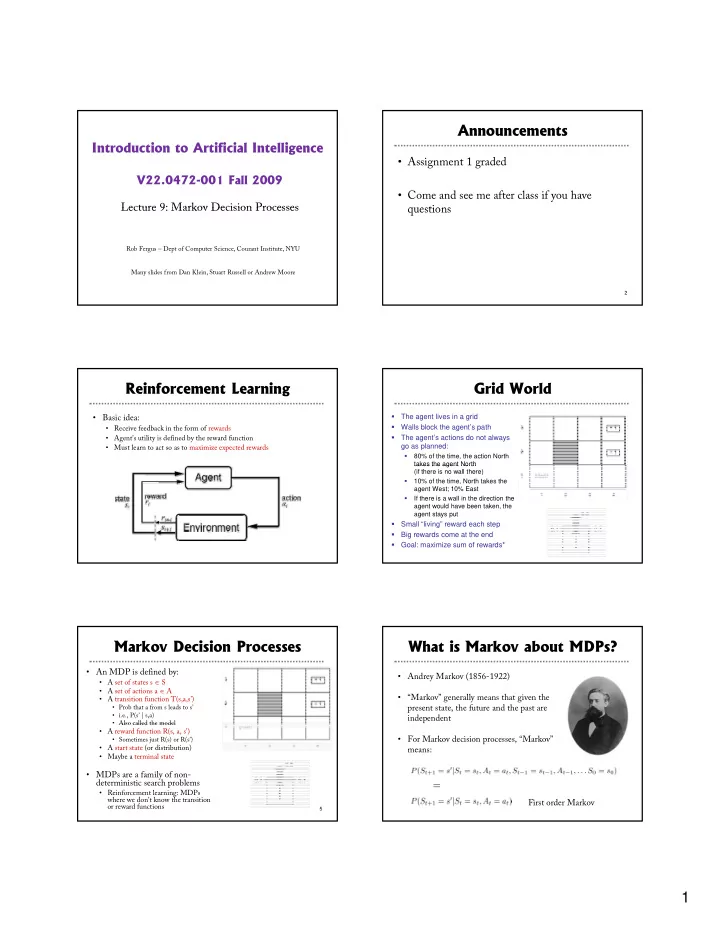
Reinforcement Learning

• Basic idea:
• Receive feedback in the form of rewards
• Agent’s utility is defined by the reward function
• Must learn to act so as to maximize expected rewards

Grid World

• The agent lives in a grid
• Walls block the agent’s path
• The agent’s actions do not always

go as planned:

• 80% of the time, the action North

takes the agent North takes the agent North (if there is no wall there)

• 10% of the time, North takes the

agent West; 10% East

• If there is a wall in the direction the

agent would have been taken, the agent stays put

• Small “living” reward each step
• Big rewards come at the end
• Goal: maximize sum of rewards*

Markov Decision Processes

• An MDP is defined by:
• A set of states s ∈ S
• A set of actions a ∈ A
• A transition function T(s,a,s’)
• Prob that a from s leads to s’
• i.e., P(s’ | s,a)
• Also called the model

Also called the model

• A reward function R(s, a, s’)
• Sometimes just R(s) or R(s’)
• A start state (or distribution)
• Maybe a terminal state
• MDPs are a family of non-

deterministic search problems

• Reinforcement learning: MDPs

where we don’t know the transition

• r reward functions

5

What is Markov about MDPs?

• Andrey Markov (1856-1922)
• “Markov” generally means that given the

present state, the future and the past are independent

• For Markov decision processes, “Markov”

means: First order Markov

2

Solving MDPs

• In deterministic single-agent search problems, want an
• ptimal plan, or sequence of actions, from start to a goal
• In an MDP, we want an optimal policy π*: S → A
• A policy π gives an action for each state
• An optimal policy maximizes expected utility if followed
• Defines a reflex agent

Optimal policy when R(s, a, s’) = -0.03 for all non-terminals s

Example Optimal Policies

8

R(s) = -2.0 R(s) = -0.4 R(s) = -0.03 R(s) = -0.01

Example: High-Low

• Three card types: 2, 3, 4
• Infinite deck, twice as many 2’s
• Start with 3 showing
• After each card, you say “high” or

“low”

• N

d i fli d

3

• New card is flipped
• If you’re right, you win the points

shown on the new card

• Ties are no-ops
• If you’re wrong, game ends
• Differences from expectimax:
• #1: get rewards as you go
• #2: you might play forever!

9

High-Low as an MDP

• States: 2, 3, 4, done
• Actions: High, Low
• Model: T(s, a, s’):
• P(s’=4 | 4, Low) = 1/4
• P(s’=3 | 4, Low) = 1/4
• P(s’=2 | 4, Low) = 1/2

3

• P(s’=done | 4, Low) = 0
• P(s’=4 | 4, High) = 1/4
• P(s’=3 | 4, High) = 0
• P(s’=2 | 4, High) = 0
• P(s’=done | 4, High) = 3/4
• …
• Rewards: R(s, a, s’):
• Number shown on s’ if s ≠ s’
• 0 otherwise
• Start: 3

Example: High-Low

Low High Low High

11

High Low High Low High Low

, Low , High T = 0.5, R = 2 T = 0.25, R = 3 T = 0, R = 4 T = 0.25, R = 0

MDP Search Trees

• Each MDP state gives an expectimax-like search tree

a s s is a state

12

s’ s, a (s,a,s’) called a transition T(s,a,s’) = P(s’|s,a) R(s,a,s’) s,a,s’ (s, a) is a q-state

3

Utilities of Sequences

• In order to formalize optimality of a policy, need to

understand utilities of sequences of rewards

• Typically consider stationary preferences:
• Theorem: only two ways to define stationary utilities
• Additive utility:
• Discounted utility:

13

Infinite Utilities?!

• Problem: infinite state sequences have infinite rewards
• Solutions:
• Finite horizon:
• Terminate episodes after a fixed T steps (e.g. life)
• Gives nonstationary policies (π depends on time left)
• Absorbing state: guarantee that for every policy, a terminal state will

eventually be reached (like “done” for High-Low)

• Discounting: for 0 < γ < 1
• Smaller γ means smaller “horizon” – shorter term focus

14

Discounting

• Typically discount

rewards by γ < 1 each time step

• Sooner rewards have

Sooner rewards have higher utility than later rewards

• Also helps the

algorithms converge

15

Recap: Defining MDPs

• Markov decision processes:
• States S
• Start state s0
• Actions A
• Transitions P(s’|s,a) (or T(s,a,s’))

a s s, a s,a,s’

• Rewards R(s,a,s’) (and discount γ)
• MDP quantities so far:
• Policy = Choice of action for each state
• Utility (or return) = sum of discounted rewards

16

, , s’

Optimal Utilities

• Fundamental operation: compute the

values (optimal expectimax utilities)

• f states s
• Why? Optimal values define optimal

policies!

• Define the al e of a state s:

a s s, a

• Define the value of a state s:

V*(s) = expected utility starting in s and acting optimally

• Define the value of a q-state (s,a):

Q*(s,a) = expected utility starting in s, taking action a and thereafter acting

• ptimally
• Define the optimal policy:

π*(s) = optimal action from state s

17

s,a,s’ s’

The Bellman Equations

• Definition of “optimal utility” leads to a

simple one-step lookahead relationship amongst optimal utility values:

Optimal rewards = maximize over first action and then follow optimal policy

a s s, a ’

and then follow optimal policy

• Formally:

18

s,a,s’ s’

4

Solving MDPs

• We want to find the optimal policy π*
• Proposal 1: modified expectimax search, starting from each

state s:

19

a s s, a s,a,s’ s’

Why Not Search Trees?

• Why not solve with expectimax?
• Problems:
• This tree is usually infinite
• Same states appear over and over
• We would search once per state

We would search once per state

• Idea: Value iteration
• Compute optimal values for all states all at
• nce using successive approximations
• Will be a bottom-up dynamic program similar

in cost to memoization

• Do all planning offline, no replanning needed!

20

Value Estimates

• Calculate estimates Vk

*(s)

• Not the optimal value of s!
• The optimal value considering
• nly next k time steps (k rewards)
• As k → ∞, it approaches the
• ptimal value
• ptimal value
• Why:
• If discounting, distant rewards

become negligible

• If terminal states reachable from

everywhere, fraction of episodes not ending becomes negligible

• Otherwise, can get infinite expected

utility and then this approach actually won’t work

21

Memoized Recursion?

• Recurrences:
• Cache all function call results so you never repeat work
• What happened to the evaluation function?

22

Value Iteration

• Problems with the recursive computation:
• Have to keep all the Vk

*(s) around all the time

• Don’t know which depth πk(s) to ask for when planning
• Solution: value iteration
• Calculate values for all states, bottom-up
• Keep increasing k until convergence

23

Value Iteration

• Idea:
• Start with V0

*(s) = 0, which we know is right (why?)

• Given Vi

*, calculate the values for all states for depth i+1:

• This is called a value update or Bellman update
• Repeat until convergence
• Theorem: will converge to unique optimal values
• Basic idea: approximations get refined towards optimal values
• Policy may converge long before values do

24

5

Example: Bellman Updates

Example: γ=0.9, living reward=0, noise=0.2 25 max happens for a=right, other actions not shown

Example: Value Iteration

V2 V3

• Information propagates outward from terminal states

and eventually all states have correct value estimates

26

[DEMO]

Convergence*

• Define the max-norm:
• Theorem: For any two approximations U and V
• I.e. any distinct approximations must get closer to each other, so, in

particular, any approximation must get closer to the true U and value iteration converges to a unique, stable, optimal solution

• Theorem:
• I.e. once the change in our approximation is small, it must also be close

to correct

27

Practice: Computing Actions

• Which action should we chose from state s:
• Given optimal values V?
• Given optimal q-values Q?
• Lesson: actions are easier to select from Q’s!

28

Recap: MDPs

• Markov decision processes:
• States S
• Actions A
• Transitions P(s’|s,a) (or T(s,a,s’))
• Rewards R(s,a,s’) (and discount γ)

a s s, a s,a,s’

• Start state s0
• Quantities:
• Returns = sum of discounted rewards
• Values = expected future returns from a state (optimal, or

for a fixed policy)

• Q-Values = expected future returns from a q-state (optimal,
• r for a fixed policy)

29

, , s’

Utilities for Fixed Policies

• Another basic operation: compute the

utility of a state s under a fixed (general non-optimal) policy

• Define the utility of a state s, under a

fixed policy π:

π(s) s s, π(s) s, π(s),s’

fixed policy π:

Vπ(s) = expected total discounted rewards (return) starting in s and following π

• Recursive relation (one-step look-ahead

/ Bellman equation):

30

s’

6

Policy Evaluation

• How do we calculate the V’s for a fixed policy?
• Idea one: modify Bellman updates
• Idea two: it’s just a linear system, solve with Matlab

(or whatever)

31

Policy Iteration

• Problem with value iteration:
• Considering all actions each iteration is slow: takes |A| times longer than

policy evaluation

• But policy doesn’t change each iteration, time wasted
• Alternative to value iteration:

Alternative to value iteration:

• Step 1: Policy evaluation: calculate utilities for a fixed policy (not optimal

utilities!) until convergence (fast)

• Step 2: Policy improvement: update policy using one-step lookahead with

resulting converged (but not optimal!) utilities (slow but infrequent)

• Repeat steps until policy converges
• This is policy iteration
• It’s still optimal!
• Can converge faster under some conditions

32

Policy Iteration

• Policy evaluation: with fixed current policy π, find values with

simplified Bellman updates:

• Iterate until values converge
• Policy improvement: with fixed utilities, find the best action

according to one-step look-ahead

33

Comparison

• In value iteration:
• Every pass (or “backup”) updates both utilities (explicitly, based on

current utilities) and policy (possibly implicitly, based on current policy)

• In policy iteration:
• In policy iteration:
• Several passes to update utilities with frozen policy
• Occasional passes to update policies
• Hybrid approaches (asynchronous policy iteration):
• Any sequences of partial updates to either policy entries or utilities will

converge if every state is visited infinitely often

34