1 2019 STAT 373/ Week 9 STAT 814_STAT714 Population values - PDF document

STAT 373/ Week 9 STAT 814_STAT714 LGAs Week 9: Example 1996 Australian Bureau of Statistics Albury, Armidale, Ashfield, Auburn, Ballina, census data Balranald, Bankstown, Barraba, Bathurst, • We will use the data from Australian Baulkham Hills, Bega Valley, Bellingen, census 1996 as an example. Berrigan, Bingara, Blacktown, …….., • Units: Local Government Areas (LGAs) of Wollongong, Woollahra, Wyong, Yallaroi, NSW (182) at the time Yarrowlumla, Yass,Young • Data are in file LGA.MTW , available on the unit iLearn. 1 2 Variables in LGA.mtw • We will be using these data to illustrate sampling and estimation techniques. Variable Mean Median Variable Mean Median Total M 18335 6997 AusBorn 13302 5991 Total F 18803 6893 AusBorn 13716 6010 • Sampling frame: list of 182 LGAs with IDs Total P 37138 13890 AusBorn 27018 12001 GE15 M 14286 5233 OSBorn M 4246 512 from 1 to 182 (N=182 LGAs) GE15 F 14944 5193 OSBorn F 4256 432 GE15 P 29231 10426 OSBorn P 8502 935 Aborig M 269.9 146.5 AusCit M 16171 6274 Aborig F 277.5 142.0 AusCit F 16599 6330 Aborig P 547.3 292.0 AusCit P 32769 12605 • We will estimate quantities such as total Unempl M 944 345 Unempl F 609.7 209.5 overseas-born population of NSW on the Unempl P 1554 586 basis of a random sample, and compare our answer with the actual total population. 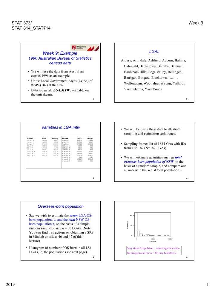3 4 Overseas-born population • Say we wish to estimate the mean LGA OS- 100 born population,  , and the total NSW OS- Frequency born population  , on the basis of a simple 50 random sample of size n = 30 LGAs. (Note: You can find instructions on obtaining a SRS in Minitab on slides 46 and 47 of this 0 0 50000 100000 lecture) OSBorn P • Histogram of number of OS-born in all 182 Very skewed population... normal approximation LGAs, ie, the population (see next page). for sample mean (for n = 30) may be unlikely. 5 6 1 2019

STAT 373/ Week 9 STAT 814_STAT714 Population values Sample (n=30) drawn using Minitab: (click Calc, Random Data, Sample from Columns and then follow it through) Descriptive Statistics LGA OS Born LGA OS Born Variable N Mean Median TrMean StDev SE Mean Tumbarumba 278 Dungog 377 Albury 3998 Bourke 162 OSBorn P 182 8502 935 5918 16237 1204 M uswellbrook 930 Pittwater 11177 Yarrowlumla 1449 Nambucca 1477 M udgee 1382 Junee 300 Variable Minimum Maximum Q1 Q3 Botany 16002 South Sydney 27729 OSBorn P 18 97203 275 8921 Hay 183 Narrabri 611 M aitland 3624 Urana 48 Great Lakes 2763 Rockdale 33491 • Mean:  = 8,502 W arringah 31893 Culcairn 227 Bland 266 M osman 7129 W agga W agga 3787 Lake M acquarie 16914 • Total:  = N  = 182×8,502=1,547,364 Crookwell 184 Kogarah 14914 Yass 879 Eurobodalla 3996 Holbrook 137 Shoalhaven 9502 7 8 Estimation of the population mean Sample Statistics Based on the sample of 30 LGAs, we have  y 6527 Descriptive Statistics  s 9713 estimated SE ( y )  s  ( 1  f ) / n 30 Variable N Mean Median TrMean StDev SE Mean   f 0.165 OSBorn s 30 6527 1463 5009 9713 1773 182 .975  t 2.0452 Variable Minimum Maximum Q1 Q3 29 OSBorn s 48 33491 275 9921 95% CI for population mean OS-born:  .975    y t s (1 f )/ n 29      6527 2.0452 9713 (1 0.165) /30  6,527  3,314  (3,213, 9,841) 9 10 Estimation of the population total NOTE: We have     y Ny 182 6527 1,187,914 • We find that the true population values of T  = 8,502 and  = 1,547,364 do in fact lie in  s 9713 large error bound;  f 0.165 the 95% confidence intervals. sample size may .975  t 2.0452 be too small. 29 • However, because of the severe skewness of 95% CI for total OS-born: the population values, it would have been  .975     y t N s (1 f )/ n T 29 more appropriate to stratify the population       1,187,914 2.0452 182 9713 (1 0.165)/30 on some criterion. [ We will return to this   1,187,914 603,175 issue later .]  (584,739,1,791,089) 11 12 2 2019

STAT 373/ Week 9 STAT 814_STAT714 Sample size required Now let’s take a SRS of size n=114 Say we wish to estimate the total OS-born in NSW within 200,000 ( = error bound) persons of the true and see what error bound we get: value, with a probability of 0.95. Descriptive Statistics Take the previous sample as a pilot study. We estimate  as s =9713. Given D = 200,000, (From Lecture 8) Variable N Mean Median TrMean StDev SE Mean C26 114 9097 935 6044 17837 1671 Then we have  1 Variable Minimum Maximum Q1 Q3   2   200000 1 C26 72 97203 275 8464    n 182  1    113 . 296    182 1 . 96 9713     Take n 114 . 13 14 We have     y Ny 182 9097 1,655,654 T Note:  s 17,837 114 • Why has the error bound turned out to be f   0.626 182 364,263 (compared to 603,175 when n = 30),  z 1.96 (as we have a large sample here) still much greater than 200,000 as planned? .975 • Recall we used s to estimate the population 95% CI for total OS-born: standard deviation  in the calculation of y  z  N s   (1  f )/ n sample size, n. T .975       1,655,654 1.96 182 17,837 (1 0.626) /114   1,655,654 364,263 15 16 We had: • If we had used the population standard deviation,  = 16,237, in the calculation of n , we would have obtained Estimate of  from pilot sample : s = 9,713 Actual value :  = 16,237 >> s  1   2 1  200000     n 182 1 149.5      182 1.96 16237       Note : The pilot sample underestimated  , which led   us to underestimate the sample size required. ie , we need n 150. 17 18 3 2019

STAT 373/ Week 9 STAT 814_STAT714 Estimating a population proportion p • We may want to estimate the – proportion/percentage (p) – number (a) Say we are interested in the presence/absence in the population that possess the of some characteristic, eg, characteristic. – person has HIV/AIDS – person watching a particular TV program A SRS of size n allows us to estimate – person supports the use of nuclear power in Australia • p = population proportion • a = Np = population total 19 20 Let Let r = number in sample with the  1 if i th member of pop n . has the characteristic u i =  characteristic of interest.  0 if i th member doesn’t have characteristic Then we estimate p by: Then    u u ... u r  1 2 N p  p ˆ N n   ( , population mean of the binary var iable u ) i and and a by       a u u ... u ( , population total ) 1 2 N N    a ˆ N ˆ p r n 21 22 Extra simplification i.e. Here u i 2 =u i since u i = 0 or 1; Thus we have • p = population mean (of the binary variable population variance worked out as follows: with values of 0 or 1)    N  2 u u i  2  i  1 • a = population total  N 1 1  N  2   2   [ u N ] NB : u , the population mean  i N 1 i  1 Good news 1  N   2 [ u N u ] i N  1 i  1 • We know properties of the estimators of N means (and totals), so we know properties  [ u  u 2 ] Recall ,   u  p  N 1 of estimators of p and a shown on Slide 21. N N      p ( 1 p ) pq , where q 1 p   N 1 N 1 23 24 4 2019