[PDF] - 1 Relation Between Multinomial Logistic Regression Nave Bayes and PDF Document

SLIDE 1

1

CS 391L: Machine Learning: Bayesian Learning: Beyond Naïve Bayes

Raymond J. Mooney

University of Texas at Austin

2

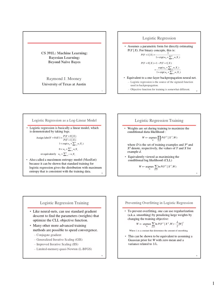
Logistic Regression

Assumes a parametric form for directly estimating

P(Y | X). For binary concepts, this is:

∑ =

+ + = =

n i i iX

w w X Y P

1

) exp( 1 1 ) | 1 (

Equivalent to a one-layer backpropagation neural net.

– Logistic regression is the source of the sigmoid function used in backpropagation. – Objective function for training is somewhat different.

) | 1 ( 1 ) | ( X Y P X Y P = − = =

∑ ∑

= =

+ + + =

n i i i n i i i

X w w X w w

1 1

) exp( 1 ) exp(

3

Logistic Regression as a Log-Linear Model

Logistic regression is basically a linear model, which

is demonstrated by taking logs.

) | 1 ( ) | ( 1 iff label Assign X Y P X Y P Y = = < =

∑ =

+ <

n i i iX

w w

1

) exp( 1

∑ =

+ <

n i i iX

w w

1

∑ = −

>

n i i iX

w w

1

ly equivalent

r
Also called a maximum entropy model (MaxEnt)

because it can be shown that standard training for logistic regression gives the distribution with maximum entropy that is consistent with the training data.

4

Logistic Regression Training

Weights are set during training to maximize the

conditional data likelihood : where D is the set of training examples and Yd and Xd denote, respectively, the values of Y and X for example d.

) , | ( argmax W X Y P W

d D d d W

∏

∈

←

Equivalently viewed as maximizing the

conditional log likelihood (CLL)

∑

∈

←

D d d d W

W X Y P W ) , | ( ln argmax

5

Logistic Regression Training

Like neural-nets, can use standard gradient

descent to find the parameters (weights) that

ptimize the CLL objective function.
Many other more advanced training

methods are possible to speed convergence.

– Conjugate gradient – Generalized Iterative Scaling (GIS) – Improved Iterative Scaling (IIS) – Limited-memory quasi-Newton (L-BFGS)

6

Preventing Overfitting in Logistic Regression

To prevent overfitting, one can use regularization

(a.k.a. smoothing) by penalizing large weights by changing the training objective:

2

2 ) , | ( ln argmax W W X Y P W

D d d d W

λ − ←

∑

∈

This can be shown to be equivalent to assuming a

Guassian prior for W with zero mean and a variance related to 1/λ.

Where λ is a constant that determines the amount of smoothing

SLIDE 2

2

7

Multinomial Logistic Regression

Logistic regression can be generalized to

multi-class problems (where Y has a multinomial distribution).

Effectively constructs a linear classifier for

each category.

8

Relation Between Naïve Bayes and Logistic Regression

Naïve Bayes with Gaussian distributions for features (GNB),

can be shown to given the same functional form for the conditional distribution P(Y|X).

– But converse is not true, so Logistic Regression makes a weaker assumption.

Logistic regression is a discriminative rather than generative

model, since it models the conditional distribution P(Y|X) and directly attempts to fit the training data for predicting Y from

X. Does not specify a full joint distribution.
When conditional independence is violated, logistic

regression gives better generalization if it is given sufficient training data.

GNB converges to accurate parameter estimates faster (O(log

n) examples for n features) compared to Logistic Regression (O(n) examples).

– Experimentally, GNB is better when training data is scarce, logistic regression is better when it is plentiful.

9

Graphical Models

If no assumption of independence is made, then an

exponential number of parameters must be estimated for sound probabilistic inference.

No realistic amount of training data is sufficient to estimate

so many parameters.

If a blanket assumption of conditional independence is made,

efficient training and inference is possible, but such a strong assumption is rarely warranted.

Graphical models use directed or undirected graphs over a

set of random variables to explicitly specify variable dependencies and allow for less restrictive independence assumptions while limiting the number of parameters that must be estimated.

– Bayesian Networks: Directed acyclic graphs that indicate causal structure. – Markov Networks: Undirected graphs that capture general dependencies.

10

Bayesian Networks

Directed Acyclic Graph (DAG)

– Nodes are random variables – Edges indicate causal influences

Burglary Earthquake Alarm JohnCalls MaryCalls

11

Conditional Probability Tables

Each node has a conditional probability table (CPT) that

gives the probability of each of its values given every possible combination of values for its parents (conditioning case).

– Roots (sources) of the DAG that have no parents are given prior probabilities. Burglary Earthquake Alarm JohnCalls MaryCalls

.001 P(B) .002 P(E) .001 F F .29 T F .94 F T .95 T T P(A) E B .01 F .70 T P(M) A .05 F .90 T P(J) A 12

CPT Comments

Probability of false not given since rows

must add to 1.

Example requires 10 parameters rather than

25–1=31 for specifying the full joint distribution.

Number of parameters in the CPT for a

node is exponential in the number of parents (fan-in).

SLIDE 3

3

13

Joint Distributions for Bayes Nets

A Bayesian Network implicitly defines a joint

distribution.

)) ( Parents | ( ) ,... , (

1 2 1 i n i i n

X x P x x x P

∏

=

Example

) ( E B A M J P ¬ ∧ ¬ ∧ ∧ ∧ ) ( ) ( ) | ( ) | ( ) | ( E P B P E B A P A M P A J P ¬ ¬ ¬ ∧ ¬ = 00062 . 998 . 999 . 001 . 7 . 9 . = × × × × =

Therefore an inefficient approach to inference is:

– 1) Compute the joint distribution using this equation. – 2) Compute any desired conditional probability using the joint distribution.

14

Naïve Bayes as a Bayes Net

Naïve Bayes is a simple Bayes Net

Y X1 X2 … Xn

Priors P(Y) and conditionals P(Xi|Y) for

Naïve Bayes provide CPTs for the network.

15

Bayes Net Inference

Given known values for some evidence variables,

determine the posterior probability of some query variables.

Example: Given that John calls, what is the

probability that there is a Burglary?

Burglary Earthquake Alarm JohnCalls MaryCalls

???

John calls 90% of the time there is an Alarm and the Alarm detects 94% of Burglaries so people generally think it should be fairly high. However, this ignores the prior probability of John calling.

16

Bayes Net Inference

Example: Given that John calls, what is the

probability that there is a Burglary?

Burglary Earthquake Alarm JohnCalls MaryCalls

???

John also calls 5% of the time when there is no Alarm. So over 1,000 days we expect 1 Burglary and John will probably

call. However, he will also call with a

false report 50 times on average. So the call is about 50 times more likely a false report: P(Burglary | JohnCalls) ≈ 0.02

.001 P(B) .05 F .90 T P(J) A 17

Bayes Net Inference

Example: Given that John calls, what is the

probability that there is a Burglary?

Burglary Earthquake Alarm JohnCalls MaryCalls

???

Actual probability of Burglary is 0.016 since the alarm is not perfect (an Earthquake could have set it off or it could have gone off on its own). On the

ther side, even if there was not an

alarm and John called incorrectly, there could have been an undetected Burglary anyway, but this is unlikely.

.001 P(B) .05 F .90 T P(J) A 18

Complexity of Bayes Net Inference

In general, the problem of Bayes Net inference is

NP-hard (exponential in the size of the graph).

For singly-connected networks or polytrees in

which there are no undirected loops, there are linear- time algorithms based on belief propagation.

– Each node sends local evidence messages to their children and parents. – Each node updates belief in each of its possible values based on incoming messages from it neighbors and propagates evidence on to its neighbors.

There are approximations to inference for general

networks based on loopy belief propagation that iteratively refines probabilities that converge to accurate values in the limit.

SLIDE 4

4

19

Belief Propagation Example

λ messages are sent from children to parents

representing abductive evidence for a node.

π messages are sent from parents to children

representing causal evidence for a node.

Burglary Earthquake Alarm JohnCalls MaryCalls

λ λ λ π

Alarm Burglary Earthquake MaryCalls

20

Markov Networks

Undirected graph over a set of random

variables, where an edge represents a dependency.

The Markov blanket of a node, X, in a

Markov Net is the set of its neighbors in the graph (nodes that have an edge connecting to X).

Every node in a Markov Net is

conditionally independent of every other node given its Markov blanket.

21

Distribution for a Markov Network

The distribution of a Markov net is most compactly

described in terms of a set of potential functions, φk, for each clique, k, in the graph.

For each joint assignment of values to the variables in

clique k, φk assigns a non-negative real value that represents the compatibility of these values.

The joint distribution of a Markov is then defined by:

) ( 1 ) ,... , (

} { 2 1

∏

=

k k k n

x Z x x x P φ Where x{k} represents the joint assignment of the variables in clique k, and Z is a normalizing constant that makes a joint distribution that sums to 1.

∑∏

=

x k k k x

Z ) (

} {

φ

22

Inference in Markov Networks

Inference in general Markov nets is #P

complete.

Approximation algorithms include:

– Markov Chain Monte Carlo (MCMC) – Loopy belief propagation

23

Bayes Nets vs. Markov Nets

Bayes nets represent a subclass of joint

distributions that capture non-cyclic causal dependencies between variables.

A Markov net can represent any joint

distribution.

– If network is fully connected then there is one clique that is includes all of the variables and whose potential function directly encodes the full joint distribution.

24

Learning Graphical Models

Structure Learning: Learn the graphical

structure of the network.

Parameter Learning: Learn the real-

valued parameters of the network

– CPTs for Bayes Nets – Potential functions for Markov Nets

SLIDE 5

5

25

Structure Learning

Use greedy top-down search through the space of

networks, considering adding each possible edge

ne at a time and picking the one that maximizes a

statistical evaluation metric that measures fit to the training data.

Alternative is to test all pairs of nodes to find ones

that are statistically correlated and adding edges accordingly.

Bayes net learning requires determining the

direction of causal influences.

Special algorithms for limited graph topologies.

– TAN (Tree Augmented Naïve-Bayes) for learning Bayes nets that are trees.

26

Parameter Learning

If values for all variables are available during

training, then parameter estimates can be directly estimated using frequency counts over the training data.

– Must smooth estimates to compensate for limited training data.

If there are hidden variables, some form of

gradient descent or Expectation Maximization (EM) must be used to estimate distributions for hidden variables.

– Like setting the weights feeding hidden units in backpropagation neural nets.

27

Statistical Relational Learning

Expand graphical model learning approach to handle

instances more expressive than feature vectors that include arbitrary numbers of objects with properties and relations between them.

– Probabilistic Relational Models (PRMs) – Stochastic Logic Programs (SLPs) – Bayesian Logic Programs (BLPs) – Relational Markov Networks (RMNs) – Markov Logic Networks (MLNs) – Other TLAs

Collective classification: Classify multiple dependent
bjects based on both and object’s properties as well as the

class of other related objects.

– Get beyond IID assumption for instances

28

Collective Classification

f Web Pages using RMNs

[Taskar, Abbeel & Koller 2002]

29

Conclusions

Bayesian learning methods are firmly based on

probability theory and exploit advanced methods developed in statistics.

Naïve Bayes is a simple generative model that works

fairly well in practice.

Logistic Regression is a discriminative classifier that

directly models the conditional distribution P(Y|X).

Graphical models allow specifying limited