1 Goals Assumptions Design a protocol that guarantees desired The - - PDF document

1

Pow er Management under Coverage and Connectivity Constraints in Sensor Netw orks

Xiaorui Wang; Guoliang Xing; Yuanfang Zhang; Chenyang Lu; Robert Pless; Christopher D. Gill Presented by: Guoliang Xing Department of Computer Science & Engineering Washington University in St Louis

2

Outline

Motivation Coverage vs. Connectivity: Geometric Analysis Coverage Configuration Protocol (CCP) Applying CCP to realistic applications Routing performance Conclusion

3

Motivation

Many sensor networks require long lifetime

Several months to years: habitat monitoring, civil structure monitoring, surveillance

Energy is scarce

Low cost energy supply, e.g., AA batteries Wireless communication is energy costly

Continuous service

Sensing Communication: network connectivity, routing ….

4

Approaches

Duty cycle schedule

Example: SMAC Cons: Long communication delay

Active backbone

Use a small number of active nodes to provide “sufficient” service Schedule other nodes to sleep Examples: SPAN, CCP

• n
• n
• ff
• ff
• ff

radio duty cycle in SMAC

Packet sent by application Packet sent to channel

5

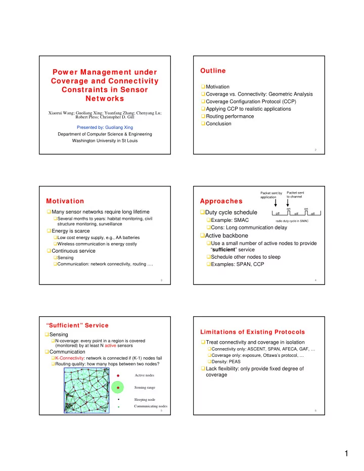
“Sufficient” Service

Sensing

N-coverage: every point in a region is covered (monitored) by at least N active sensors

Communication

K-Connectivity: network is connected if (K-1) nodes fail Routing quality: how many hops between two nodes?

Sleeping node Communicating nodes Active nodes Sensing range

6

Limitations of Existing Protocols

Treat connectivity and coverage in isolation

Connectivity only: ASCENT, SPAN, AFECA, GAF, … Coverage only: exposure, Ottawa’s protocol, … Density: PEAS

Lack flexibility: only provide fixed degree of coverage

2

7

Goals

Design a protocol that guarantees desired coverage and connectivity Requirements

Integrated: must guarantee both coverage and connectivity Flexible: can re-configure the network to different coverage degrees and connectivity

Meet diverse application requirements

Decentralized: achieve scalability

8

Assumptions

The region to be covered is convex Disc models for coverage and communication A point p is covered by a node v if |pv| < Rs Rs: Sensing range Nodes u and v are connected if |uv| < Rc Rc: Communication range Intuition: range ratio Rc/Rs is important!

Rc Rs

9

Outline

Motivation Coverage vs. Connectivity: Geometric Analysis Coverage Configuration Protocol (CCP) Simulation results Routing performance Conclusion

10

Connectivity vs. Coverage

A connected network does not guarantee coverage

Connectivity only concerns with node locations Coverage must cover all locations in a region True for any Rc/Rs

If Rc/Rs ≥ 2

K-coverage K-connectivity for all nodes K-coverage 2K-connectivity for interior nodes

Interior node: a node whose sensing circle fully contained by the region

11

Implication of Geometric Analysis

Given a required coverage degree of Ks, and a required connectivity of Kc If Rc ≥ 2Rs, the protocol only needs to guarantee max(Ks. Kc) coverage configuration

Solution: Coverage Configuration Protocol (CCP)

If Rc < 2Rs, the protocol must address both coverage and connectivity.

Solution: CCP + SPAN

12

A Sufficient Condition for K-Coverage

A convex region B is K-covered if all the intersection points among sensing circles and/or B’s boundary inside B are K-covered Implication: a coverage configuration protocol only needs to worry about intersection points!

S

p

Intuition: All points in a same “patch” surrounded by sensing circles share the same coverage degree

Assumption: boundary of each circle is not covered by the sensor

3

13

K-Coverage Eligibility Rule

All intersection points inside the sensing circle are K-covered?

To evaluate eligibility, a node only needs to know the locations of active nodes within 2Rs

Active nodes Sleeping nodes Intersection point

• n?

14

Coverage Configuration Protocol (CCP) Active nodes periodically broadcast and receive beacon messages Sleeping nodes periodically wake up and receive beacons Change state based on the eligibility rule

Active sleeping if the eligibility rule is true Sleeping active if the eligibility rule is false

15

Simulation: Coverage Configurability

2 4 6 8 10 1 2 3 4 5 6 7 Required Coverage degree Achieved Coverage degree Min-500,700,900 Average-500 Average-700 Average-900

CCP strictly enforces desired coverage degrees!

16

CCP+SPAN

When Rc < 2Rs, CCP cannot guarantee connectivity. Solution: CCP + SPAN Combined eligibility rule

Sleeping active if either CCP or SPAN activates the node Active sleeping if both CCP and SPAN put the node to sleep

17

SPAN

All nodes periodically broadcast/receive beacons Change state based on the eligibility rule

Active sleeping if the eligibility rule is false Sleeping active if the eligibility rule is true

Eligibility rule:

At least one pair of my neighbors cannot reach each

• ther either directly or via one or two active nodes?

Every sleeping node is within one hop of at least

• ne active node

18

Simulation: Coverage+Connectivity (Rc = 1.5Rs)

Combination of SPAN & CCP is necessary for desired coverage and connectivity when Rc < 2Rs SPAN CCP SPAN+CCP

4

19

Simulation: Coverage vs Rc/Rs

0.2 0.4 0.6 0.8 1 0.5 1 1.5 2 2.5 3 Coverage Percentage Rc/Rs Coverage Percentage CCP-2Hop SPAN+CCP-2Hop CCP SPAN+CCP SPAN

CCP-based protocols guarantee coverage for all Rc/Rs SPAN’s cannot guarantee coverage for any Rc/Rs

20

Simulation: Connectivity vs Rc/Rs

0.1 0.2 0.3 0.4 0.5 0.6 0.7 0.8 0.9 1 1.1 0.5 1 1.5 2 2.5 3 Packet delivery ratio Rc/Rs Packet Delivery Ratio CCP-2Hop SPAN+CCP-2Hop CCP SPAN+CCP SPAN

SPAN-based protocols delivers more packets CCP cannot delivery all packets when Rc/Rs < 2

21

System LifeTime

0.1 0.2 0.3 0.4 0.5 0.6 0.7 0.8 0.9 1 100 200 300 400 500 600 700 800 900 1000 1100 Coverage Percentage Time System Coverage Life (Rc/Rs=2.5) SPAN+CCP-300 Original-300 SPAN+CCP-250 Original-250 SPAN+CCP-200 Original-200 0.4 0.5 0.6 0.7 0.8 0.9 1 1.1 100 200 300 400 500 600 700 800 9 Delivery Ratio Time System Communication Life (Rc/Rs=2.5) SPAN+CCP-300 Original-300 SPAN+CCP-250 Original-250 Original-200 SPAN+CCP-200

22

Outline

Motivation Coverage vs. Connectivity: Geometric Analysis Coverage Configuration Protocol (CCP) Applying CCP to realistic applications Routing performance Conclusion

23

Realistic Detection Applications

Requirements: detection prob., false alarm rate Probabilistic sensing range

Stochastic signals/noises Signal decay Usually determined from empirical measurements

Multi-sensor data fusion

Single sensor may be faulty and cause false alarms Reliable detection decision should base on multiple sensor readings Fusion rule: how to reach a final decision based on multiple sensor readings?

24

Applying CCP to Realistic Detection Applications Probabilistic sensing model

A point within the sensing rang of a sensor is covered with prob. P

Application requirement: (K, β) coverage

Prob(target is detected)≥ β Target detected if sensed by at least K sensors

Solution: run CCP with coverage degree K’ given by:

∑

− = − ′

≥ − ⎟ ⎟ ⎠ ⎞ ⎜ ⎜ ⎝ ⎛ ′ −

1

) 1 ( 1

s s

K i i K i s

P P i K β

5

25

Illustration: Applying CCP to Realistic Detection Applications The prob. is sensed by 2 sensors must > 0.95 Each sensor senses with prob. 0.9 How many sensors are needed to cover ? P=0.9, K=2, β=0.95, K’=?

Target Sensing range

26

Scalability and Performance

1 2 3 4 5 6 7 8 9 10 11 12 13 14 15 16 17 18 1 2 3 4 5 6 7 8 9 10 11 Lower Bound of Psudo Coverage Degree Ks Lower Bound of Psudo Coverage Degree vs. Ks P=0.7 P=0.8 P=0.9

1 2 3 4 5 6 7 8 9 10 11 1 2 3 4 5 6 7 Ks

*

Ks Ks

* vs. Ks (P=0.8)

• Avg. (β=0.80)
• Avg. (β=0.90)
• Avg. (β=0.95)
• Min. (β=0.85)
• Min. (β=0.90)
• Min. (β=0.95)

β=0.95

27

Outline

Motivation Coverage vs. Connectivity: Geometric Analysis Coverage Configuration Protocol (CCP) Applying CCP to realistic applications Routing performance Conclusion

28

Impact of Sensing Coverage on Routing Performance

Sensing coverage results in a special class of topologies

Coverage Node density/geometric properties

How do they affect routing performance?

Existing routing algorithms perform better? Can a routing algorithm take advantage of the network properties imposed by coverage?

29

Greedy Geographic Forw arding

• Forward packet to the neighbor with the shortest

distance to destination A destination

shortest Euclidean distance to destination

B

30

Pros and Cons of Greedy Forw arding

Local decision based on neighbor locations

Allow efficient implementation on constrained platforms Match location-centric communication paradigm in WSN

Fail when a packet reaches a local minima A node cannot find a neighbor better than itself Recovery schemes: face routing, flooding Result in long routes

• Does greedy geo-routing perform better on

sensing-covered networks?

• Can we establish analytical performance

bounds?

6

31

Routing Metric: Netw ork Dilation

Network dilation of a graph under a routing algorithm Definition Low Dn means good routing algorithm For any two nodes u and v, a path no longer than Dn hops can be found by a routing algorithm whose network dilation is Dn

⎥ ⎥ ⎤ ⎢ ⎢ ⎡ =

∈ c V v u n

R uv v u D | | ) , ( max

,

τ

min # of hops # of hops found by a routing algorithm

⎥ ⎥ ⎤ ⎢ ⎢ ⎡

c

R uv | | 32

Advance at least Rc-2Rs Always include a node due to coverage

Greedy Forw arding in Netw orks w ith Coverage

GF always succeeds when Rc/Rs > 2 # of hops between u and v:

s c

R R uv 2 | | −

Rc

No advance when Rc 2 Rs

33

Do Better than Greedy Geo-routing

Voronoi Diagram of a set of nodes V partitions the plane into Voronoi regions, one for each node.

A point lies inside u’s Voronoi region iff u is the closest node to the point.

Delauney Triangulation (DT) is the dual graph of Voronoi diagram of V

An edge between u and v in DT iff Vor(u) and Vor(v) share a boundary The Euclidean distance of shortest path from u to v in DT < 2.42 |uv|

Theorem: DT is a sub-graph of the network with sensing coverage

Good routing algorithm is possible by taking advantage of DT

34

Bounded Voronoi Greedy Forw arding (BVGF)

A neighbor is eligible only if its Voronoi region intersects the line joining source and destination Greedy: choose the eligible neighbor closest to destination

eligible not eligible

35

1 1.5 2 2.5 3 3.5 4 4.5 5 5.5 6 6.5 7 7.5 8 8.5 9 9.5 10 2 2.5 3 3.5 4 4.5 5 5.5 6 6.5 7 7.5 8 8.5 9 9.5 10 Network Dilation Rc/Rs Network Dilation vs. Rc/Rs GF Asymptotic Bound BVGF Asymptotic Bound DT Bound GF BVGF

Asymptotic Netw ork Dilation

62 . 4 3 3 8 max ≈ =

BVGF bound

36

Conclusion

Geometric analysis on relationship between coverage and connectivity

Only need to worry about coverage when Rc ≥ 2Rs: Coverage Configuration Protocol Must worry about both when Rc < 2Rs: CCP + SPAN

CCP can be applied to realistic applications Sensing coverage implies good routing property

Simple greedy geo-routing works well Justifies power management protocols that maintain sensing coverage

Source can compute bound on network distance based

• n source/destination locations

Scalable real-time communication

7

37

Critiques

Circular sensing/communication range Need more realistic sensing model (see CoGrid paper: www.cs.wustl.edu/~xing) Geometric routing may not work well when communication links are unreliable No evaluation on motes