1 t=1 t=2 t=1 t=2 $100 $100 $80 $80 $60 $60 $80 - - PDF document

1

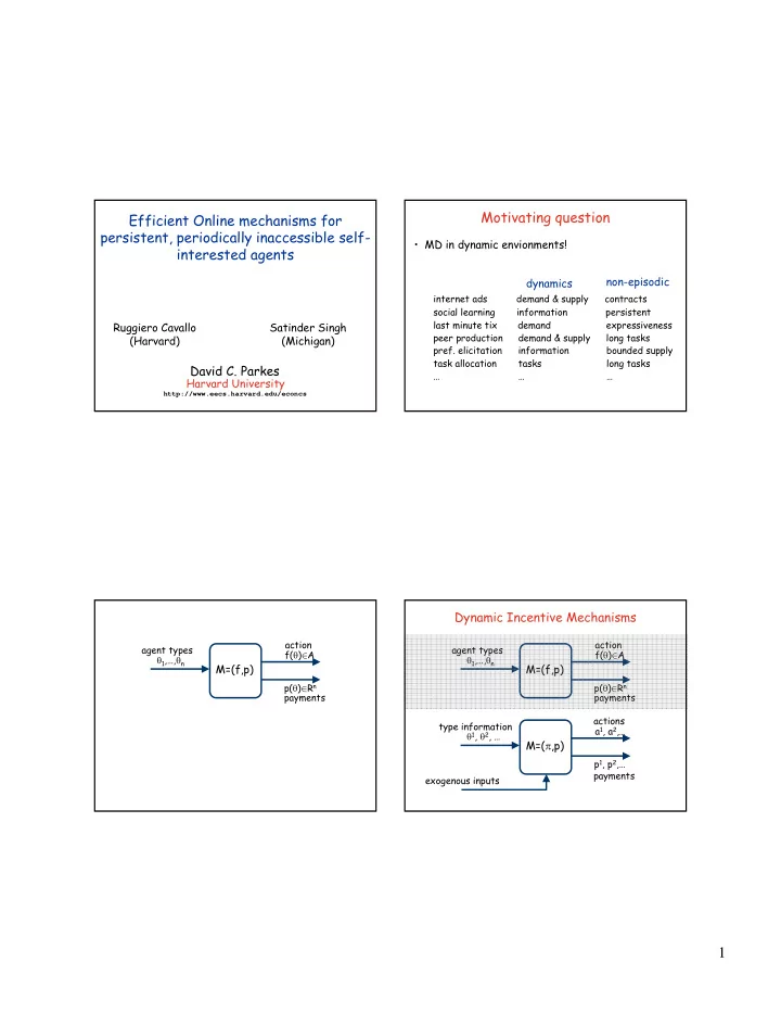
Efficient Online mechanisms for persistent, periodically inaccessible self- interested agents

David C. Parkes

Harvard University

http://www.eecs.harvard.edu/econcs

Ruggiero Cavallo (Harvard) Satinder Singh (Michigan)

Motivating question

• MD in dynamic envionments!

dynamics non-episodic

internet ads demand & supply contracts social learning information persistent last minute tix demand expressiveness peer production demand & supply long tasks

• pref. elicitation

information bounded supply task allocation tasks long tasks … … … agent types θ1,…,θn f(θ)∈A p(θ)∈Rn

M=(f,p)

action payments type information θ1, θ2, … a1, a2,… p1, p2,…

M=(π,p)

actions payments exogenous inputs agent types θ1,…,θn f(θ)∈A p(θ)∈Rn

M=(f,p)

action payments

Dynamic Incentive Mechanisms

2

$100 $80 t=1 t=2

… …

$60 $100 $80 $60 t=1 t=2 $80

… …

$100 $80 $60 t=1 t=2 $80 $60

… … One view from CS

• Prior free:
• Typical setting: (ei,di,vi,qi)
• Body of work

– Lavi & Nisan ’00 – Awerbuch et al. ’03 – Porter ’04 – Hajiaghayi, Kleinberg, Parkes’04 – Blum & Hartline ’05 – Hajiaghayi, Kleinberg, Mahdian, Parkes’05 – Lavi & Nisan ’05 – …

• DSIC, monotonicity-based characterizations

3

One view from CS

• Prior free:
• Typical setting: (ei,di,vi,qi)
• Body of work

– Lavi & Nisan ’00 – Awerbuch et al. ’03 – Porter ’04 – Hajiaghayi, Kleinberg, Parkes’04 – Blum & Hartline ’05 – Hajiaghayi, Kleinberg, Mahdian, Parkes’05 – Lavi & Nisan ’05 – …

• DSIC, monotonicity-based characterizations.
• Limited misreports: no-early arrival, no-late dep., etc.

A second view

• Center (and/or agents) have a probabilistic model of

dynamics of environment

• π*(s)∈ arg maxa [r(s,a) +γ ∑s’∈St+1 Pr(s’,a,s)V*(s’)]
• Agents can misreport local model, local state
• Body of work:

– Parkes & Singh ’03, ’04 – Cavallo, Parkes & Singh ’06 – Bergemann and Valamaki ’06 – Cavallo, Parkes & Singh ’07 – …

• typically interim IC, sometimes DSIC

A second view

• Center (and/or agents) have a probabilistic model of

dynamics of environment

• π*(s)∈ arg maxa [r(s,a) +γ ∑s’∈St+1 Pr(s’,a,s)V*(s’)]
• Agents can misreport local model, local state
• Body of work:

– Parkes & Singh ’03, ’04 – Cavallo, Parkes & Singh ’06 – Bergemann and Valimaki ’06 – Cavallo, Parkes & Singh ’07 – Athey & Segal ’07

• typically interim IC, sometimes DSIC

type = static component (local model)

4

type = static component (local model) + dynamic component (local state) type = static component (local model) + dynamic component (local state) type = static component (local model) + dynamic component (local state) type = static component (local model) + dynamic component (local state)

5

type = static component (local model) + dynamic component (local state) type = static component (local model) + dynamic component (local state) type = static component (local model) + dynamic component (local state) type = static component (local model) + dynamic component (local state)

6

• Dynamic types, persistent agents
• Dynamic types, arrival + departures
• Dynamic types, accessible/inaccessible

MDP: (Si,A,ri,τi) τi(si,a) ri(si,a) initial state si policy πi: Si→ A Vπ

i(s)=E[∑k=t γk-trk i(sk i,π(sk))]

V*

i(s): π* i ∈ arg maxπ Vπ i(s)

…

S=S0 × S1 ×… × Sn r(s,a)=∑iri(si,a) τ=(τ0,τ1,…,τn) τ0(s0,a) a∈A(s)

…

policy π: S→ A Vπ(s)=E[∑k=t γk-trk(sk,π(sk))] V*(s): π*∈ arg maxπ Vπ(s) MDP: (Si,A,ri,τi) τi(si,a) ri(si,a) initial state si policy πi: Si→ A Vπ

i(s)=E[∑k=t γk-trk i(sk i,π(sk))]

V*

i(s): π* i ∈ arg maxπ Vπ i(s)

S=S0 × S1 ×… × Sn r(s,a)=∑iri(si,a) τ=(τ0,τ1,…,τn) τ0(s0,a) a∈A(s)

…

policy π: S→ A Vπ(s)=E[∑k=t γk-trk(sk,π(sk))] V*(s): π*∈ arg maxπ Vπ(s) MDP: (Si,A,ri,τi) τi(si,a) ri(si,a) initial state si policy πi: Si→ A Vπ

i(s)=E[∑k=t γk-trk i(sk i,π(sk))]

V*

i(s): π* i ∈ arg maxπ Vπ i(s)

Assumption: CIA

(Conditional Independence given Actions)

ri((si,s-i),a)=ri((si,s-i’),a) τi((si,s-i),a)=τi((si,s-i’),a)

7

Example: Coordinated learning … … … … … …

payment: V*(s-i) – V*(s-i | π*(s) ) ⇒ interim IC (in every state)

(CPS’06,BV’06)

report states report models actions π*(st) collect payments period t strategy: history × type → report S=S0 × S1 ×… × Sn r(s,a)=∑iri(si,a) τ=(τ0,τ1,…,τn) a∈A(s)

…

policy π: S→ A Vπ(s)=E[∑k=t γk-trk(sk,π(sk))] V*(s): π*∈ arg maxπ Vπ(s) A == {public|voluntary|private}

standard in MD OK if observable private effects

report states report models actions π*(st) make/suggest

• bserve

actions collect payments period t

8

• Dynamic types, persistent agents
• Dynamic types, arrival + departures
• Dynamic types, accessible/inaccessible

…

arrival/departure process

…

arrival/departure process

…

arrival/departure process

9

…

arrival/departure process

…

arrival/departure process

…

arrival/departure process

static type == (local model,initial state) H(s0): set of static types present s=(s0, {si}i∈H(s0))∈S τ0: S0 × A → S0 r(s,a)=∑i∈H(s0)ri(si,a) arrival process

…

departure: local absorbing state

10

Special case: Deterministic Local Models

• Only dynamics are arrival/departure of static types
• Agents arrive and declare reward for all future

sequences of actions via deterministic local model

…

alloc 5 alloc 5 alloc 5 alloc alloc alloc alloc alloc alloc 5 100 linear valuation all-or-nothing unit-demand

static type == (local model,initial state) H(s0): set of static types present s=(s0, {si}i∈H(s0))∈S τ0: S0 × A → S0 r(s,a)=∑i∈H(s0)ri(si,a) Assumption: CIA

Conditional Independence given Actions

Pr(θt | θ1..t-1,a1..t-1)=Pr(θt|a1..t-1) arrival process

…

departure: local absorbing state

• Dynamic types, persistent agents
• Dynamic types, arrival + departures
• Dynamic types, accessible/inaccessible

arrival/depature = inaccess → access → inaccess

11

• Augment local state with accessible/inaccessible
• Inaccessible == no messages, no payments
• Can pretend to be inaccessible when not

accessible (but not vice versa)

• Actions can make an agent become inaccessible
• Can have reward for actions while inaccessible
• Assumption: run but can’t hide // pay the piper
• Augment local state with accessible/inaccessible
• Inaccessible == no messages, no payments
• Can pretend to be inaccessible when not

accessible (but not vice versa)

• Actions can make an agent become inaccessible
• Can have reward for actions while inaccessible
• Assumption: run but can’t hide // pay the piper

A Belief-state MDP model

• Partially Observable Markov Decision Process
• Model as a belief-state MDP (Kaelbling et al. 96)

– BS=S0× BS1× … × BSn , BSi=∆(Si) – when accessible, bsi∈ BSi, reduces to point mass – ri(bsi

ta): in expectation on underlying states

– policy π*: BS → A Persistent & Dynamic type CIA: r(si,a) τ(si,a) BV’06 V*

• i(s)-V*
• i(s|π*(s))

charge each period Arr/dep & Static type r(si,a) τ(si,a) Pr(θt|θ1..t−1,a1..t-1)=Pr(θt|a1..t-1) PS’03 vi-(V*(se)-V*(se

• i))

charge @ departure Persistent, Access/inaccess, dynamic type r(si,a) τ(si,a) RBCH CPS’07 charge where δt is # periods been inaccessible Arr/dep & Dynamic type r(si,a) τ(si,a) Pr(θt|θ1..t−1,a1..t-1)=Pr(θt|a1..t-1) CPS’07 V*

• i(s)-V*
• i(s|π*(s))

charge each period

12

• Expected equilibrium payoff to agent i is

V∗(st|fi)–Ci(st), where Ci(st) is independent of strategy fi

• persistent: in every state
• arrival/departure: in arrival period
• access/inaccess: in every accessible state
• Groves intuition: agent i’s payoff is aligned with

expected true value of policy, maximizes this by reporting true type given that policy π is optimal

• Expected equilibrium payoff to agent i is

V∗(st|fi)–Ci(st), where Ci(st) is independent of strategy fi

• persistent: in every state
• arrival/departure: in arrival period
• access/inaccess: in every accessible state
• Groves intuition: agent i’s payoff is aligned with

expected true value of policy, maximizes this by reporting true type given that policy π is optimal

• Subtle: V*(st) – V*(st-i) does not work!

Relating to “Offline VCG”

• ffline VCG
• optimal x* // DSIC
• ex post IR
• ex post ND

need private values dynamic VCG

• optimal π* // interim IC
• interim IR (V*(st)≥V*
• i(st
• i))
• interim ND (V*
• i(st
• i)≥V*
• i(st))

ε−correctness of model ε−optimality of policy critical for incentive properties

Computational issues

• Special cases will be feasible to solve offline, e.g. via

value or policy iteration. Payments come from Q-values.

• Local Markov chains (Gittins’74)

– discounting & infinite time horizon – activate agent with maximal index

• In general, large (even continuous) state space. Need
• nline sample-approximation methods.
• Tree-sampling (Kearns, Mansour & Ng’99, Ng & Jordan’00)

– applied to online MD by Parkes & Singh’04 – scale exponentially in number of actions and look-ahead, but independent of state space – ε-optimality and ε-equilibrium

• Trajectory-sampling (van Hentenryck et al.)

– suitable in deterministic local model // independent arrival process setting – avoids exponential scaling, but hard to prove bounds (but see Mercier, Upfal & van Hentenryck ’07)

13

Computational issues

• Special cases will be feasible to solve offline, e.g. via

value or policy iteration. Payments come from Q-values.

• Local Markov chains (Gittins’74)

– discounting & infinite time horizon – activate agent with maximal index

• In general, large (even continuous) state space. Need
• nline sample-approximation methods.
• Tree-sampling (Kearns, Mansour & Ng’99, Ng & Jordan’00)

– applied to online MD by Parkes & Singh’04 – scale exponentially in number of actions and look-ahead, but independent of state space – ε-optimality and ε-equilibrium

• Trajectory-sampling (van Hentenryck et al.)

– suitable in deterministic local model // independent arrival process setting – avoids exponential scaling, but hard to prove bounds (but see Mercier, Upfal & van Hentenryck ’07)

Computational issues

• Special cases will be feasible to solve offline, e.g. via

value or policy iteration. Payments come from Q-values.

• Local Markov chains (Gittins’74)

– discounting & infinite time horizon – activate agent with maximal index

• In general, large (even continuous) state space. Need
• nline sample-approximation methods.
• Tree-sampling (Kearns, Mansour & Ng’99, Ng & Jordan’00)

– applied to online MD by Parkes & Singh’04 – scale exponentially in number of actions and look-ahead, but independent of state space – ε-optimality and ε-equilibrium

• Trajectory-sampling (van Hentenryck et al.)

– suitable in deterministic local model // independent arrival process setting – avoids exponential scaling, but hard to prove bounds (but see Mercier, Upfal & van Hentenryck ’07)

Computational issues

• Special cases will be feasible to solve offline, e.g. via

value or policy iteration. Payments come from Q-values.

• Local Markov chains (Gittins’74)

– discounting & infinite time horizon – activate agent with maximal index

• In general, large (even continuous) state space. Need
• nline sample-approximation methods.
• Tree-sampling (Kearns, Mansour & Ng’99, Ng & Jordan’00)

– applied to online MD by Parkes & Singh’04 – scale exponentially in number of actions and look-ahead, but independent of state space – ε-optimality and ε-equilibrium (poly in 1/ε)

• Trajectory-sampling (van Hentenryck et al.)

– suitable in deterministic local model // independent arrival process setting – avoids exponential scaling, but hard to prove bounds (but see Mercier, Upfal & van Hentenryck ’07)

Computational issues

• Special cases will be feasible to solve offline, e.g. via

value or policy iteration. Payments come from Q-values.

• Local Markov chains (Gittins’74)

– discounting & infinite time horizon – activate agent with maximal index

• In general, large (even continuous) state space. Need
• nline sample-approximation methods.
• Tree-sampling (Kearns, Mansour & Ng’99, Ng & Jordan’00)

– applied to online MD by Parkes & Singh’04 – scale exponentially in number of actions and look-ahead, but independent of state space – ε-optimality and ε-equilibrium (poly in 1/ε)

• Trajectory-sampling (van Hentenryck et al.)

– suitable in deterministic local model // independent arrival process setting – avoids exponential scaling, but hard to prove bounds (but see Mercier, Upfal & van Hentenryck ’07)

14

Parallel literature: DSIC

• set-valued setting (e,d,r,L)
• limited misreports and/or delayed allocation and

late departures

• makes monotonicity in sense of earlier arrival,

later departure, smaller L sufficient competitive analysis

• nline stochastic

combinatorial optimization + “output ironing”

(Parkes&Duong, Constantin&Parkes)

Parallel literature: DSIC

• set-valued setting (e,d,r,L)
• limited misreports and/or delayed allocation and

late departures

• makes monotonicity in sense of earlier arrival,

later departure, smaller L sufficient competitive analysis

• nline stochastic

combinatorial optimization + “output ironing”

(Parkes&Duong, Constantin&Parkes)

Open problems Indirect methods

• Direct revelation of type information costly, and

counter to privacy concerns

• Prefer to allow agents to retain private model,

perform local planning, report enough information to allow optimal joint actions

• Look for price-based methods

15

Cashless design

• What about dynamic coordination in systems

without money?

• Dynamic voting protocols
• c.f. Jackson “linking mechanism”

Richer models, Economic Qs

• Two-sided models, e.g. dynamic (combinatorial)
• exchanges. Only have results for simple settings.

E.g., Blum et al.’06, Parkes & Bredin’07

• Redistribution methods. Can the methods of

Bailey, Cavallo, Guo & Conitzer, Moulin, Hartline

• etc. be leveraged?
• What about revenue?
• Learning by center?
• etc…

Approximate incentive compatibility

• Likely will need to relax IC requirements
• One approach

– have local agents help with computation – suggest improved policies – fold new computational methods into the mechanism – c.f. Nisan & Ronen (second-chance) – c.f. Cavallo (belief-coordination mechanism)

• Another approach

– local stability – first price vs. generalized second price vs. GSP, Threshold rule, etc. – tolerable manipulability

Applications/Comput. Directions

• Meta-deliberation auctions

– use these techniques to coordinate the deliberation process of agents – extend MD to embrace more of the process of decision making

• Online CAs

– obvious application area – lots of algorithmic challenges

• AI architectures

– can this be used to coordinate computational processes?

16

• Rich agenda in embracing dynamics within

mechanism design

• Relevant to many kinds of coordination

problems, including computational processes

• Fun new challenges ☺

Summary

www.eecs.harvard.edu/econcs