1 Prior Work Stereology Prior Work Stereology Prior Work - PDF document

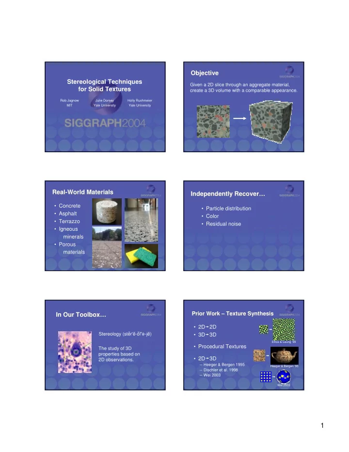
Objective Objective Stereological Techniques Given a 2D slice through an aggregate material, for Solid Textures create a 3D volume with a comparable appearance. Rob Jagnow Julie Dorsey Holly Rushmeier MIT Yale University Yale University Real-World Materials Real-World Materials Independently Recover… Independently Recover… • Concrete • Particle distribution • Asphalt • Color • Terrazzo • Residual noise • Igneous minerals • Porous materials Prior Work – Texture Synthesis Prior Work – Texture Synthesis In Our Toolbox… In Our Toolbox… • 2D 2D Stereology (ster'e-ol ' -je) e • 3D 3D Efros & Leung ’99 • Procedural Textures The study of 3D properties based on • 2D 3D 2D observations. – Heeger & Bergen 1995 Heeger & Bergen ’95 – Dischler et al. 1998 – Wei 2003 Wei 2003 1

Prior Work – Stereology Prior Work – Stereology Prior Work – Texture Synthesis Prior Work – Texture Synthesis • Saltikov 1967 Particle size distributions from section measurements • Underwood 1970 Quantitative Stereology • Howard and Reed 1998 Unbiased Stereology • Wojnar 2002 Stereology from one of all the possible angles Input Heeger & Bergen, ’95 Recovering Sphere Distributions Recovering Sphere Distributions Recovering Sphere Distributions Recovering Sphere Distributions N = Profile density Group profiles and particles into n bins A (number of circles per unit area) according to diameter N = Particle density V ≤ ≤ (number of spheres per unit volume) Particle densities = N A ( i ), { 1 i n } ≤ ≤ = Mean caliper particle diameter Profile densities = N V ( i ), { 1 i n } H The fundamental relationship of stereology: For the following examples, n = 4 N = H N A V Recovering Sphere Distributions Recovering Sphere Distributions Recovering Sphere Distributions Recovering Sphere Distributions How many profiles of the largest size? Note that the profile source is ambiguous = N ( 4 ) K N ( 4 ) A 44 V K = Probability that particle N V ( j ) exhibits profile N A ( i ) ij 2

Recovering Sphere Distributions Recovering Sphere Distributions Recovering Sphere Distributions Recovering Sphere Distributions Putting it all together… How many profiles of the smallest size? = + + + = N ( 1 ) K N ( 1 ) K N ( 2 ) K N ( 3 ) K N ( 4 ) A 11 V 12 V V V 13 14 K = Probability that particle N V ( j ) exhibits profile N A ( i ) ij N K N A V Recovering Sphere Distributions Recovering Sphere Distributions Recovering Sphere Distributions Recovering Sphere Distributions = Some minor rearrangements… N d KN A max V K is upper-triangular and invertible N K N = d A V max For spheres, we can solve for K analytically: ( ) ⎧ ⎪ ⋅ − − − − j ≥ 2 2 2 2 for i 1 / n j ( i 1 ) j i d = Maximum diameter = ⎨ K ij max ⎪ ⎩ 0 otherwise Normalize probabilities for each column j : n ∑ = = − 1 1 K j / n Solving for particle densities: N K N ij V d A = max i 1 Other Particle Types Other Particle Types Testing precision Testing precision We cannot classify arbitrary particles by d/d max Input Instead, we choose to use A / A distribution max Estimated Algorithm inputs: distribution + Approach: Collect statistics for 2D profiles and 3D particles 3

Profile Statistics Profile Statistics Particle Statistics Particle Statistics Look at thousands of Segment input image to obtain profile densities N A . random slices to obtain H and K 0.45 0.4 sphere cube 0.35 long ellipsoid flat ellipsoid 0.3 Example probabilities of probability 0.25 for simple particles 0.2 A / A max Input Segmentation 0.15 i l p r o b a b t y i 0.1 0.05 0 Bin profiles according to their area, A / A 0.1 0.2 0.3 0.4 0.5 0.6 0.7 0.8 0.9 1 max A / A max Recovering Color Recovering Color Recovering Particle Distributions Recovering Particle Distributions Select mean particle colors from N = Just like before, H KN A V segmented regions in the input image Solving for the particle densities, = − 1 1 N K N V A H Use N V to populate a synthetic volume. Input Mean Colors Synthetic Volume Recovering Noise Recovering Noise Putting it all together Putting it all together How can we replicate the noisy appearance of the input? - = Input Mean Colors Residual The noise residual is less Input structured and responds well to Heeger & Bergen’s method Synthetic volume with noise Synthesized Residual 4

Prior Work – Revisited Prior Work – Revisited Results – Physical Data Results – Physical Data Input Heeger & Bergen ’95 Our result Physical Heeger & Our Model Bergen ’95 Method Results Results Results Results Input Result Input Result Summary Summary Future Work Future Work • Particle distribution • Automated particle construction – Stereological techniques • Extend technique to other domains and • Color anisotropic appearances – Mean colors of segmented profiles • Perceptual analysis of results • Residual noise – Replicated using Heeger & Bergen ’95 5

Thanks to… Thanks to… • Maxwell Planck, undergraduate assistant • Virginia Bernhardt • Bob Sumner • John Alex 6