[PDF] - 1 Bayes Theorem Bayesian Categorization Determine category of x k PDF Document

SLIDE 1

1

CS 391L: Machine Learning: Bayesian Learning: Naïve Bayes

Raymond J. Mooney

University of Texas at Austin

2

Axioms of Probability Theory

All probabilities between 0 and 1
True proposition has probability 1, false has

probability 0. P(true) = 1 P(false) = 0.

The probability of disjunction is:

1 ) ( ≤ ≤ A P ) ( ) ( ) ( ) ( B A P B P A P B A P ∧ − + = ∨

A B

B A∧

3

Conditional Probability

P(A | B) is the probability of A given B
Assumes that B is all and only information

known.

Defined by:

) ( ) ( ) | ( B P B A P B A P ∧ =

A B

B A∧

4

Independence

A and B are independent iff:
Therefore, if A and B are independent:

) ( ) | ( A P B A P = ) ( ) | ( B P A B P =

) ( ) ( ) ( ) | ( A P B P B A P B A P = ∧ =

) ( ) ( ) ( B P A P B A P = ∧

These two constraints are logically equivalent

5

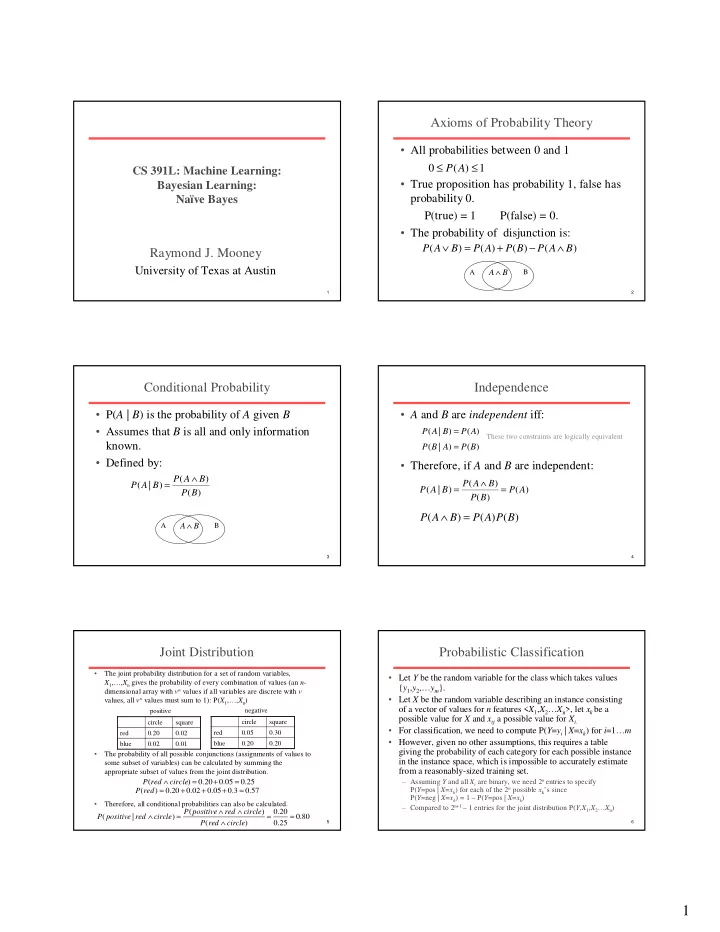
Joint Distribution

The joint probability distribution for a set of random variables,

X1,…,Xn gives the probability of every combination of values (an n- dimensional array with vn values if all variables are discrete with v values, all vn values must sum to 1): P(X1,…,Xn)

The probability of all possible conjunctions (assignments of values to

some subset of variables) can be calculated by summing the appropriate subset of values from the joint distribution.

Therefore, all conditional probabilities can also be calculated.

0.01 0.02 blue 0.02 0.20 red square circle 0.20 0.20 blue 0.30 0.05 red square circle positive negative

25 . 05 . 20 . ) ( = + = ∧ circle red P 80 . 25 . 20 . ) ( ) ( ) | ( = = ∧ ∧ ∧ = ∧ circle red P circle red positive P circle red positive P 57 . 3 . 05 . 02 . 20 . ) ( = + + + = red P

6

Probabilistic Classification

Let Y be the random variable for the class which takes values

{y1,y2,…ym}.

Let X be the random variable describing an instance consisting
f a vector of values for n features <X1,X2…Xn>, let xk be a

possible value for X and xij a possible value for Xi.

For classification, we need to compute P(Y=yi | X=xk) for i=1…m
However, given no other assumptions, this requires a table

giving the probability of each category for each possible instance in the instance space, which is impossible to accurately estimate from a reasonably-sized training set.

– Assuming Y and all Xi are binary, we need 2n entries to specify P(Y=pos | X=xk) for each of the 2n possible xk’s since P(Y=neg | X=xk) = 1 – P(Y=pos | X=xk) – Compared to 2n+1 – 1 entries for the joint distribution P(Y,X1,X2…Xn)

SLIDE 2

2

7

Bayes Theorem

Simple proof from definition of conditional probability:

) ( ) ( ) | ( ) | ( E P H P H E P E H P = ) ( ) ( ) | ( E P E H P E H P ∧ = ) ( ) ( ) | ( H P E H P H E P ∧ = ) ( ) | ( ) ( H P H E P E H P = ∧ QED:

(Def. cond. prob.) (Def. cond. prob.)

) ( ) ( ) | ( ) | ( E P H P H E P E H P =

8

Bayesian Categorization

Determine category of xk by determining for each yi
P(X=xk) can be determined since categories are

complete and disjoint.

) ( ) | ( ) ( ) | (

k i k i k i

x X P y Y x X P y Y P x X y Y P = = = = = = =

∑ ∑

= =

= = = = = = = =

m i k i k i m i k i

x X P y Y x X P y Y P x X y Y P

1 1

1 ) ( ) | ( ) ( ) | (

∑

=

= = = = =

m i i k i k

y Y x X P y Y P x X P

1

) | ( ) ( ) (

9

Bayesian Categorization (cont.)

Need to know:

– Priors: P(Y=yi) – Conditionals: P(X=xk | Y=yi)

P(Y=yi) are easily estimated from data.

– If ni of the examples in D are in yi then P(Y=yi) = ni / |D|

Too many possible instances (e.g. 2n for binary

features) to estimate all P(X=xk | Y=yi).

Still need to make some sort of independence

assumptions about the features to make learning tractable.

10

Generative Probabilistic Models

Assume a simple (usually unrealistic) probabilistic method

by which the data was generated.

For categorization, each category has a different

parameterized generative model that characterizes that category.

Training: Use the data for each category to estimate the

parameters of the generative model for that category.

– Maximum Likelihood Estimation (MLE): Set parameters to maximize the probability that the model produced the given training data. – If Mλ denotes a model with parameter values λ and Dk is the training data for the kth class, find model parameters for class k (λk) that maximize the likelihood of Dk:

Testing: Use Bayesian analysis to determine the category

model that most likely generated a specific test instance. ) | ( argmax

λ λ

λ M D P

k k =

11

Naïve Bayes Generative Model

Size Color Shape Size Color Shape

Positive Negative

pos neg pos pos pos neg neg sm med lg lg med sm sm med lg red red red red red blue blue grn circ circ circ circ sqr tri tri circ sqr tri sm lg med sm lg med lg sm blue red grn blue grn red grn blue circ sqr tri circ sqr circ tri

Naïve Bayes Inference Problem

Size Color Shape Size Color Shape

Positive Negative

pos neg pos pos pos neg neg sm med lg lg med sm sm med lg red red red red red blue blue grn circ circ circ circ sqr tri tri circ sqr tri sm lg med sm lg med lg sm blue red grn blue grn red grn blue circ sqr tri circ sqr circ tri

Category lg red circ

?? ??

SLIDE 3

3

13

Naïve Bayesian Categorization

If we assume features of an instance are independent given

the category (conditionally independent).

Therefore, we then only need to know P(Xi | Y) for each

possible pair of a feature-value and a category.

If Y and all Xi and binary, this requires specifying only 2n

parameters:

– P(Xi=true | Y=true) and P(Xi=true | Y=false) for each Xi – P(Xi=false | Y) = 1 – P(Xi=true | Y)

Compared to specifying 2n parameters without any

independence assumptions.

) | ( ) | , , ( ) | (

1 2 1

∏

=

= =

n i i n

Y X P Y X X X P Y X P L

14

Naïve Bayes Example

15

Naïve Bayes Example

16

Estimating Probabilities

Normally, probabilities are estimated based on observed

frequencies in the training data.

If D contains nk examples in category yk, and nijk of these nk

examples have the jth value for feature Xi, xij, then:

However, estimating such probabilities from small training

sets is error-prone.

If due only to chance, a rare feature, Xi, is always false in

the training data, ∀yk :P(Xi=true | Y=yk) = 0.

If Xi=true then occurs in a test example, X, the result is that

∀yk: P(X | Y=yk) = 0 and ∀yk: P(Y=yk | X) = 0

k ijk k ij i

n n y Y x X P = = = ) | (

17

Probability Estimation Example

negitive triangle red small 3 positive circle red large 2 positive circle red small 1 negitive circle blue large 4 Category Shape Color Size Ex

Test Instance X: <medium, red, circle> P(positive | X) = 0.5 * 0.0 * 1.0 * 1.0 / P(X) = 0 P(negative | X) = 0.5 * 0.0 * 0.5 * 0.5 / P(X) = 0

18

Smoothing

To account for estimation from small samples,

probability estimates are adjusted or smoothed.

Laplace smoothing using an m-estimate assumes that

each feature is given a prior probability, p, that is assumed to have been previously observed in a “virtual” sample of size m.

For binary features, p is simply assumed to be 0.5.

m n mp n y Y x X P

k ijk k ij i

+ + = = = ) | (

SLIDE 4

4

19

Laplace Smothing Example

Assume training set contains 10 positive examples:

– 4: small – 0: medium – 6: large

Estimate parameters as follows (if m=1, p=1/3)

– P(small | positive) = (4 + 1/3) / (10 + 1) = 0.394 – P(medium | positive) = (0 + 1/3) / (10 + 1) = 0.03 – P(large | positive) = (6 + 1/3) / (10 + 1) = 0.576 – P(small or medium or large | positive) = 1.0

20

Continuous Attributes

If Xi is a continuous feature rather than a discrete one, need

another way to calculate P(Xi | Y).

Assume that Xi has a Gaussian distribution whose mean

and variance depends on Y.

During training, for each combination of a continuous

feature Xi and a class value for Y, yk, estimate a mean, µik , and standard deviation σik based on the values of feature Xi in class yk in the training data.

During testing, estimate P(Xi | Y=yk) for a given example,

using the Gaussian distribution defined by µik and σik .

        − − = =

2 2

2 ) ( exp 2 1 ) | (

ik ik i ik k i

X y Y X P σ µ π σ

21

Comments on Naïve Bayes

Tends to work well despite strong assumption of

conditional independence.

Experiments show it to be quite competitive with other

classification methods on standard UCI datasets.

Although it does not produce accurate probability

estimates when its independence assumptions are violated, it may still pick the correct maximum-probability class in many cases.

– Able to learn conjunctive concepts in any case

Does not perform any search of the hypothesis space.

Directly constructs a hypothesis from parameter estimates that are easily calculated from the training data.

– Strong bias

Not guarantee consistency with training data.
Typically handles noise well since it does not even focus
n completely fitting the training data.