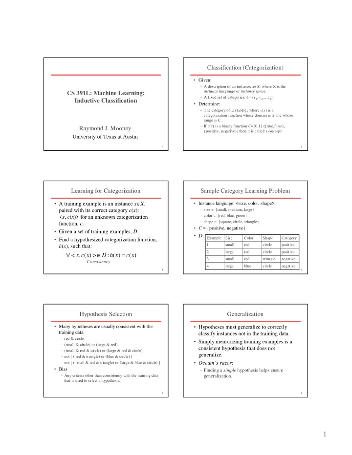
1 Hypothesis Space Inductive Learning Hypothesis Restrict learned - - PDF document

SLIDE 1

1

1

CS 391L: Machine Learning: Inductive Classification Raymond J. Mooney

University of Texas at Austin

2

Classification (Categorization)

• Given:

– A description of an instance, x∈X, where X is the instance language or instance space. – A fixed set of categories: C={c1, c2,…cn}

• Determine:

– The category of x: c(x)∈C, where c(x) is a categorization function whose domain is X and whose range is C. – If c(x) is a binary function C={0,1} ({true,false}, {positive, negative}) then it is called a concept.

3

Learning for Categorization

• A training example is an instance x∈X,

paired with its correct category c(x): <x, c(x)> for an unknown categorization function, c.

• Given a set of training examples, D.
• Find a hypothesized categorization function,

h(x), such that:

) ( ) ( : ) ( , x c x h D x c x = ∈ > < ∀

Consistency

4

Sample Category Learning Problem

• Instance language: <size, color, shape>

– size ∈ {small, medium, large} – color ∈ {red, blue, green} – shape ∈ {square, circle, triangle}

• C = {positive, negative}
• D:

negative triangle red small 3 positive circle red large 2 positive circle red small 1 negative circle blue large 4 Category Shape Color Size Example

5

Hypothesis Selection

• Many hypotheses are usually consistent with the

training data.

– red & circle – (small & circle) or (large & red) – (small & red & circle) or (large & red & circle) – not [ ( red & triangle) or (blue & circle) ] – not [ ( small & red & triangle) or (large & blue & circle) ]

• Bias

– Any criteria other than consistency with the training data that is used to select a hypothesis.

6

Generalization

• Hypotheses must generalize to correctly

classify instances not in the training data.

• Simply memorizing training examples is a

consistent hypothesis that does not generalize.

• Occam’s razor:

– Finding a simple hypothesis helps ensure generalization.

SLIDE 2

2

7

Hypothesis Space

• Restrict learned functions a priori to a given hypothesis

space, H, of functions h(x) that can be considered as definitions of c(x).

• For learning concepts on instances described by n discrete-

valued features, consider the space of conjunctive hypotheses represented by a vector of n constraints <c1, c2, … cn> where each ci is either:

– ?, a wild card indicating no constraint on the ith feature – A specific value from the domain of the ith feature – Ø indicating no value is acceptable

• Sample conjunctive hypotheses are

– <big, red, ?> – <?, ?, ?> (most general hypothesis) – < Ø, Ø, Ø> (most specific hypothesis)

8

Inductive Learning Hypothesis

• Any function that is found to approximate the target

concept well on a sufficiently large set of training examples will also approximate the target function well on unobserved examples.

• Assumes that the training and test examples are drawn

independently from the same underlying distribution.

• This is a fundamentally unprovable hypothesis unless

additional assumptions are made about the target concept and the notion of “approximating the target function well

• n unobserved examples” is defined appropriately (cf.

computational learning theory).

9

Evaluation of Classification Learning

• Classification accuracy (% of instances

classified correctly).

– Measured on an independent test data.

• Training time (efficiency of training

algorithm).

• Testing time (efficiency of subsequent

classification).

10

Category Learning as Search

• Category learning can be viewed as searching the

hypothesis space for one (or more) hypotheses that are consistent with the training data.

• Consider an instance space consisting of n binary features

which therefore has 2n instances.

• For conjunctive hypotheses, there are 4 choices for each

feature: Ø, T, F, ?, so there are 4n syntactically distinct hypotheses.

• However, all hypotheses with 1 or more Øs are equivalent,

so there are 3n+1 semantically distinct hypotheses.

• The target binary categorization function in principle could

be any of the possible 22^n functions on n input bits.

• Therefore, conjunctive hypotheses are a small subset of the

space of possible functions, but both are intractably large.

• All reasonable hypothesis spaces are intractably large or

even infinite.

11

Learning by Enumeration

• For any finite or countably infinite hypothesis

space, one can simply enumerate and test hypotheses one at a time until a consistent one is found.

• ✁

✂ ✄ ☎ ✆ ✝ ✞ ✟ ✠ ✡ ☛ ✁ ☞ ✌ ✍ ✞ ✟ ✎ ✆ ✁ ✠ ✎ ✟ ✎ ✏ ✄ ✠ ✏ ✑ ✟ ✏ ✝ ✏ ✝ ✄ ✏ ✂ ☎ ✟ ✠ ✟ ✠ ✒ ☛ ☎ ✏ ☎ ✓ ✔ ✏ ✝ ✄ ✠ ✏ ✄ ✂ ✕ ✟ ✠ ☎ ✏ ✄ ☎ ✠ ☛ ✂ ✄ ✏ ✖ ✂ ✠ ✞ ✗

• This algorithm is guaranteed to terminate with a

consistent hypothesis if one exists; however, it is

• bviously computationally intractable for almost

any practical problem.

12

Efficient Learning

• Is there a way to learn conjunctive concepts

without enumerating them?

• How do human subjects learn conjunctive

concepts?

• Is there a way to efficiently find an

unconstrained boolean function consistent with a set of discrete-valued training instances?

• If so, is it a useful/practical algorithm?

SLIDE 3

3

13

Conjunctive Rule Learning

• Conjunctive descriptions are easily learned by finding

all commonalities shared by all positive examples.

• Must check consistency with negative examples. If

inconsistent, no conjunctive rule exists.

negative triangle red small 3 positive circle red large 2 positive circle red small 1 negative circle blue large 4 Category Shape Color Size Example

Learned rule: red & circle → positive

14

Limitations of Conjunctive Rules

• If a concept does not have a single set of necessary

and sufficient conditions, conjunctive learning fails.

negative circle blue large 4 negative triangle red small 3 positive circle red large 2 positive circle red small 1 negative circle red medium 5 Category Shape Color Size Example

Learned rule: red & circle → positive Inconsistent with negative example #5!

15

Disjunctive Concepts

• Concept may be disjunctive.

negative circle blue large 4 negative triangle red small 3 positive circle red large 2 positive circle red small 1 negative circle red medium 5 Category Shape Color Size Example

Learned rules: small & circle → positive large & red → positive

16

Using the Generality Structure

• By exploiting the structure imposed by the generality of

hypotheses, an hypothesis space can be searched for consistent hypotheses without enumerating or explicitly exploring all hypotheses.

• An instance, x∈X, is said to satisfy an hypothesis, h, iff

h(x)=1 (positive)

• Given two hypotheses h1 and h2, h1 is more general than
• r equal to h2 (h1≥h2) iff every instance that satisfies h2

also satisfiesh1.

• Given two hypotheses h1 and h2, h1 is (strictly) more

general than h2 (h1>h2) iff h1≥h2 and it is not the case that h2 ≥ h1.

• Generality defines a partial order on hypotheses.

17

Examples of Generality

• Conjunctive feature vectors

– <?, red, ?> is more general than <?, red, circle> – Neither of <?, red, ?> and <?, ?, circle> is more general than the other.

• Axis-parallel rectangles in 2-d space

– A is more general than B – Neither of A and C are more general than the other.

A B C

18

Sample Generalization Lattice

< Ø, Ø, Ø> <?,?,circ> <big,?,?> <?,red,?> <?,blue,?> <sm,?,?> <?,?,squr> < big,red,circ><sm,red,circ><big,blue,circ><sm,blue,circ>< big,red,squr><sm,red,squr><big,blue,squr><sm,blue,squr> < ?,red,circ><big,?,circ><big,red,?><big,blue,?><sm,?,circ><?,blue,circ> <?,red,squr><sm.?,sqr><sm,red,?><sm,blue,?><big,?,squr><?,blue,squr> <?, ?, ?>

Size: {sm, big} Color: {red, blue} Shape: {circ, squr} Number of hypotheses = 33 + 1 = 28

SLIDE 4

4

19

Most Specific Learner (Find-S)

• Find the most-specific hypothesis (least-general generalization,

LGG) that is consistent with the training data.

• Incrementally update hypothesis after every positive example,

generalizing it just enough to satisfy the new example.

• For conjunctive feature vectors, this is easy:

✘ ✙ ✚ ✛ ✚ ✜ ✢ ✚ ✣ ✤ ✥ ✦ ✧ ★ ✩ ★ ✩ ✪ ★ ✫ ✬ ✭ ✮ ✤ ✜ ✯ ✰ ✱ ✭ ✲ ✚ ✛ ✚ ✳ ✤ ✛ ✮ ✜ ✚ ✙ ✚ ✙ ✴ ✚ ✙ ✲ ✛ ✜ ✙ ✯ ✤ ✵ ✚ ✙ ✶ ✬ ✭ ✮ ✤ ✜ ✯ ✰ ✷ ✤ ✜ ✛ ✸ ✮ ✤ ✷ ✹ ✘ ✷ ✛ ✰ ✤ ✯ ✭ ✙ ✲ ✛ ✮ ✜ ✚ ✙ ✛ ✭ ✙ ✷ ✹ ✚ ✙ ✥ ✚ ✲ ✺ ✻ ✼ ✲ ✜ ✛ ✚ ✲ ✷ ✚ ✤ ✽ ✾ ✿ ✵ ✘ ✷ ✷ ✹ ✚ ✙ ✥ ✚ ✲ ★ ✛ ✰ ✤ ✙ ✲ ✤ ✛ ✷ ✹ ✚ ✙ ✥ ✛ ✭ ✛ ✰ ✤ ✳ ✜ ✢ ✸ ✤ ✭ ✷ ✷ ✹ ✚ ✙ ✵ ✤ ✢ ✲ ✤ ✲ ✤ ✛ ✷ ✹ ✚ ✙ ✥ ✛ ✭ ❀ ❁ ❂ ✘ ✷ ✥ ✚ ✲ ✯ ✭ ✙ ✲ ✚ ✲ ✛ ✤ ✙ ✛ ❃ ✚ ✛ ✰ ✛ ✰ ✤ ✙ ✤ ✴ ✜ ✛ ✚ ✳ ✤ ✛ ✮ ✜ ✚ ✙ ✚ ✙ ✴ ✚ ✙ ✲ ✛ ✜ ✙ ✯ ✤ ✲ ✚ ✙ ✶ ✛ ✰ ✤ ✙ ✮ ✤ ✛ ✸ ✮ ✙ ✥ ✤ ✢ ✲ ✤ ✙ ✭ ✯ ✭ ✙ ✲ ✚ ✲ ✛ ✤ ✙ ✛ ✰ ✿ ✱ ✭ ✛ ✰ ✤ ✲ ✚ ✲ ✤ ❄ ✚ ✲ ✛ ✲

Time complexity: O(|D| n) if n is the number

• f features

20

Properties of Find-S

• For conjunctive feature vectors, the most-specific

hypothesis is unique and found by Find-S.

• If the most specific hypothesis is not consistent

with the negative examples, then there is no consistent function in the hypothesis space, since, by definition, it cannot be made more specific and retain consistency with the positive examples.

• For conjunctive feature vectors, if the most-

specific hypothesis is inconsistent, then the target concept must be disjunctive.

21

Another Hypothesis Language

• Consider the case of two unordered objects each described

by a fixed set of attributes.

– {<big, red, circle>, <small, blue, square>}

• What is the most-specific generalization of:

– Positive: {<big, red, triangle>, <small, blue, circle>} – Positive: {<big, blue, circle>, <small, red, triangle>}

• LGG is not unique, two incomparable generalizations are:

– {<big, ?, ?>, <small, ?, ?>} – {<?, red, triangle>, <?, blue, circle>}

• For this space, Find-S would need to maintain a

continually growing set of LGGs and eliminate those that cover negative examples.

• Find-S is no longer tractable for this space since the

number of LGGs can grow exponentially.

22

Issues with Find-S

• Given sufficient training examples, does Find-S converge

to a correct definition of the target concept (assuming it is in the hypothesis space)?

• How de we know when the hypothesis has converged to a

correct definition?

• Why prefer the most-specific hypothesis? Are more

general hypotheses consistent? What about the most- general hypothesis? What about the simplest hypothesis?

• If the LGG is not unique

– Which LGG should be chosen? – How can a single consistent LGG be efficiently computed or determined not to exist?

• What if there is noise in the training data and some training

examples are incorrectly labeled?

23

Effect of Noise in Training Data

• Frequently realistic training data is corrupted by errors

(noise) in the features or class values.

• Such noise can result in missing valid generalizations.

– For example, imagine there are many positive examples like #1 and #2, but out of many negative examples, only one like #5 that actually resulted from a error in labeling.

negative circle blue large 4 negative triangle red small 3 positive circle red large 2 positive circle red small 1 negative circle red medium 5 Category Shape Color Size Example

24

Version Space

• Given an hypothesis space, H, and training

data, D, the version space is the complete subset of H that is consistent with D.

• The version space can be naively generated

for any finite H by enumerating all hypotheses and eliminating the inconsistent

• nes.
• Can one compute the version space more

efficiently than using enumeration?

SLIDE 5

5

25

Version Space with S and G

• The version space can be represented more compactly by

maintaining two boundary sets of hypotheses, S, the set of most specific consistent hypotheses, and G, the set of most general consistent hypotheses:

• S and G represent the entire version space via its boundaries in

the generalization lattice:

)]} , ( [ ) , ( | { D s Consistent s s H s D s Consistent H s S ′ ∧ ′ > ∈ ′ ¬∃ ∧ ∈ = )]} , ( [ ) , ( | { D s Consistent g g H g D g Consistent H g G ′ ∧ > ′ ∈ ′ ¬∃ ∧ ∈ =

version space G S

26

Version Space Lattice

< Ø, Ø, Ø> <?,?,circ> <big,?,?> <?,red,?> <?,blue,?> <sm,?,?> <?,?,squr> < big,red,circ><sm,red,circ><big,blue,circ><sm,blue,circ>< big,red,squr><sm,red,squr><big,blue,squr><sm,blue,squr> < ?,red,circ><big,?,circ><big,red,?><big,blue,?><sm,?,circ><?,blue,circ> <?,red,squr><sm.?,sqr><sm,red,?><sm,blue,?><big,?,squr><?,blue,squr> <?, ?, ?>

Size: {sm, big} Color: {red, blue} Shape: {circ, squr} <<big, red, squr> positive> <<sm, blue, circ> negative> Color Code: G S

• ther VS

27

Candidate Elimination (Version Space) Algorithm

Initialize G to the set of most-general hypotheses in H Initialize S to the set of most-specific hypotheses in H For each training example, d, do: If d is a positive example then: Remove from G any hypotheses that do not match d For each hypothesis s in S that does not match d Remove s from S Add to S all minimal generalizations, h, of s such that: 1) h matches d 2) some member of G is more general than h Remove from S any h that is more general than another hypothesis in S If d is a negative example then: Remove from S any hypotheses that match d For each hypothesis g in G that matches d Remove g from G Add to G all minimal specializations, h, of g such that: 1) h does not match d 2) some member of S is more specific than h Remove from G any h that is more specific than another hypothesis in G

28

Required Subroutines

• To instantiate the algorithm for a specific

hypothesis language requires the following procedures:

– equal-hypotheses(h1, h2) – more-general(h1, h2) – match(h, i) – initialize-g() – initialize-s() – generalize-to(h, i) – specialize-against(h, i)

29

Minimal Specialization and Generalization

• Procedures generalize-to and specialize-against

are specific to a hypothesis language and can be complex.

• For conjunctive feature vectors:

– generalize-to: unique, see Find-S – specialize-against: not unique, can convert each “?” to an alernative non-matching value for this feature.

• Inputs:

– h = <?, red, ?> – i = <small, red, triangle>

• Outputs:

– <big, red, ?> – <medium, red, ?> – <?, red, square> – <?, red, circle>

30

Sample VS Trace

S= {< Ø, Ø, Ø>}; G= {<?, ?, ?>} Positive: <big, red, circle> Nothing to remove from G Minimal generalization of only S element is <big, red, circle> which is more specific than G. S={<big, red, circle>}; G={<?, ?, ?>} Negative: <small, red, triangle> Nothing to remove from S. Minimal specializations of <?, ?, ?> are <medium, ?, ?>, <big, ?, ?>, <?, blue, ?>, <?, green, ?>, <?, ?, circle>, <?, ?, square> but most are not more general than some element of S S={<big, red, circle>}; G={<big, ?, ?>, <?, ?, circle>}

SLIDE 6

6

31

Sample VS Trace (cont)

S={<big, red, circle>}; G={<big, ?, ?>, <?, ?, circle>} Positive: <small, red, circle> Remove <big, ?, ?> from G Minimal generalization of <big, red, circle> is <?, red, circle> S={<?, red, circle>}; G={<?, ?, circle>} Negative: <big, blue, circle> Nothing to remove from S Minimal specializations of <?, ?, circle> are <small, ? circle>, <medium, ?, circle>, <?, red, circle>, <?, green, circle> but most are not more general than some element of S. S={<?, red, circle>}; G={<?, red, circle>} S=G; Converged!

32

Properties of VS Algorithm

• S summarizes the relevant information in the positive

examples (relative to H) so that positive examples do not need to be retained.

• G summarizes the relevant information in the negative

examples, so that negative examples do not need to be retained.

• Result is not affected by the order in which examples are

processes but computational efficiency may.

• Positive examples move the S boundary up; Negative

examples move the G boundary down.

• If S and G converge to the same hypothesis, then it is the
• nly one in H that is consistent with the data.
• If S and G become empty (if one does the other must also)

then there is no hypothesis in H consistent with the data.

33

Sample Weka VS Trace 1

java weka.classifiers.vspace.ConjunctiveVersionSpace -t figure.arff -T figure.arff -v -P Initializing VersionSpace S = [[#,#,#]] G = [[?,?,?]] Instance: big,red,circle,positive S = [[big,red,circle]] G = [[?,?,?]] Instance: small,red,square,negative S = [[big,red,circle]] G = [[big,?,?], [?,?,circle]] Instance: small,red,circle,positive S = [[?,red,circle]] G = [[?,?,circle]] Instance: big,blue,circle,negative S = [[?,red,circle]] G = [[?,red,circle]] Version Space converged to a single hypothesis.

34

Sample Weka VS Trace 2

java weka.classifiers.vspace.ConjunctiveVersionSpace -t figure2.arff -T figure2.arff -v -P Initializing VersionSpace S = [[#,#,#]] G = [[?,?,?]] Instance: big,red,circle,positive S = [[big,red,circle]] G = [[?,?,?]] Instance: small,blue,triangle,negative S = [[big,red,circle]] G = [[big,?,?], [?,red,?], [?,?,circle]] Instance: small,red,circle,positive S = [[?,red,circle]] G = [[?,red,?], [?,?,circle]] Instance: medium,green,square,negative S = [[?,red,circle]] G = [[?,red,?], [?,?,circle]]

35

Sample Weka VS Trace 3

java weka.classifiers.vspace.ConjunctiveVersionSpace -t figure3.arff -T figure3.arff -v -P Initializing VersionSpace S = [[#,#,#]] G = [[?,?,?]] Instance: big,red,circle,positive S = [[big,red,circle]] G = [[?,?,?]] Instance: small,red,triangle,negative S = [[big,red,circle]] G = [[big,?,?], [?,?,circle]] Instance: small,red,circle,positive S = [[?,red,circle]] G = [[?,?,circle]] Instance: big,blue,circle,negative S = [[?,red,circle]] G = [[?,red,circle]] Version Space converged to a single hypothesis. Instance: small,green,circle,positive S = [] G = [] Language is insufficient to describe the concept.

36

Sample Weka VS Trace 4

java weka.classifiers.vspace.ConjunctiveVersionSpace -t figure4.arff -T figure4.arff -v -P Initializing VersionSpace S = [[#,#,#]] G = [[?,?,?]] Instance: small,red,square,negative S = [[#,#,#]] G = [[medium,?,?], [big,?,?], [?,blue,?], [?,green,?], [?,?,circle], [?,?,triangle]] Instance: big,blue,circle,negative S = [[#,#,#]] G = [[medium,?,?], [?,green,?], [?,?,triangle], [big,red,?], [big,?,square], [small,blue,?], [?,blue,square], [small,?,circle], [?,red,circle]] Instance: big,red,circle,positive S = [[big,red,circle]] G = [[big,red,?], [?,red,circle]] Instance: small,red,circle,positive S = [[?,red,circle]] G = [[?,red,circle]] Version Space converged to a single hypothesis.

SLIDE 7

7

37

Correctness of Learning

• Since the entire version space is maintained, given

a continuous stream of noise-free training examples, the VS algorithm will eventually converge to the correct target concept if it is in the hypothesis space, H, or eventually correctly determine that it is not in H.

• Convergence is correctly indicated when S=G.

38

Computational Complexity of VS

• Computing the S set for conjunctive feature

vectors is linear in the number of features and the number of training examples.

• Computing the G set for conjunctive feature

vectors is exponential in the number of training examples in the worst case.

• In more expressive languages, both S and G can

grow exponentially.

• The order in which examples are processed can

significantly affect computational complexity.

39

Active Learning

• In active learning, the system is responsible for

selecting good training examples and asking a teacher (oracle) to provide a class label.

• In sample selection, the system picks good

examples to query by picking them from a provided pool of unlabeled examples.

• In query generation, the system must generate the

description of an example for which to request a label.

• Goal is to minimize the number of queries

required to learn an accurate concept description.

40

Active Learning with VS

• An ideal training example would eliminate half of the

hypotheses in the current version space regardless of its label.

• If a training example matches half of the hypotheses in the

version space, then the matching half is eliminated if the example is negative, and the other (non-matching) half is eliminated if the example is positive.

• Example:

– Assume training set

• Positive: <big, red, circle>
• Negative: <small, red, triangle>

– Current version space:

• {<big, red, circle>, <big, red, ?>, <big, ?, circle>, <?, red, circle>

<?, ?, circle> <big, ?, ?>} – An optimal query: <big, blue, circle>

• Given a ceiling of log2|VS| such examples will result in
• convergence. This is the best possible guarantee in general.

41

Using an Unconverged VS

• If the VS has not converged, how does it classify a novel

test instance?

• If all elements of S match an instance, then the entire

version space much (since it is more general) and it can be confidently classified as positive (assuming target concept is in H).

• If no element of G matches an instance, then the entire

version space must not (since it is more specific) and it can be confidently classified as negative (assuming target concept is in H).

• Otherwise, one could vote all of the hypotheses in the VS

(or just the G and S sets to avoid enumerating the VS) to give a classification with an associated confidence value.

• Voting the entire VS is probabilistically optimal assuming

the target concept is in H and all hypotheses in H are equally likely a priori.

42

Learning for Multiple Categories

• What if the classification problem is not concept learning

and involves more than two categories?

• Can treat as a series of concept learning problems, where

for each category, Ci, the instances of Ci are treated as positive and all other instances in categories Cj, j≠i are treated as negative (one-versus-all).

• This will assign a unique category to each training instance

but may assign a novel instance to zero or multiple categories.

• If the binary classifier produces confidence estimates (e.g.

based on voting), then a novel instance can be assigned to the category with the highest confidence.

• Other approaches exist, such as learning to discriminate all

pairs of categories (all-pairs) and combining decisions appropriately during test.

SLIDE 8

8

43

Inductive Bias

• A hypothesis space that does not include all possible

classification functions on the instance space incorporates a bias in the type of classifiers it can learn.

• Any means that a learning system uses to choose between

two functions that are both consistent with the training data is called inductive bias.

• Inductive bias can take two forms:

– Language bias: The language for representing concepts defines a hypothesis space that does not include all possible functions (e.g. conjunctive descriptions). – Search bias: The language is expressive enough to represent all possible functions (e.g. disjunctive normal form) but the search algorithm embodies a preference for certain consistent functions

• ver others (e.g. syntactic simplicity).

44

Unbiased Learning

• For instances described by n features each with m values, there are

mn instances. If these are to be classified into c categories, then there are cm^n possible classification functions. – For n=10, m=c=2, there are approx. 3.4x1038 possible functions, of which only 59,049 can be represented as conjunctions (an incredibly small percentage!)

• However, unbiased learning is futile since if we consider all possible

functions then simply memorizing the data without any real generalization is as good an option as any.

• Without bias, the version-space is always trivial. The unique most-

specific hypothesis is the disjunction of the positive instances and the unique most general hypothesis is the negation of the disjunction of the negative instances:

)} ... ( { )} ... {(

2 1 2 1 j k

n n n G p p p S ∨ ∨ ∨ ¬ = ∨ ∨ ∨ =

45

Futility of Bias-Free Learning

• A learner that makes no a priori assumptions about the

target concept has no rational basis for classifying any unseen instances.

• Inductive bias can also be defined as the assumptions that,

when combined with the observed training data, logically entail the subsequent classification of unseen instances.

– Training-data + inductive-bias |― novel-classifications

• The bias of the VS algorithm (assuming it refuses to

classify an instance unless it is classified the same by all members of the VS), is simply that H contains the target concept.

• The rote learner, which refuses to classify any instance

unless it has seen it during training, is the least biased.

• Learners can be partially ordered by their amount of bias

– Rote-learner < VS Algorithm < Find-S

46

No Panacea

• No Free Lunch (NFL) Theorem (Wolpert, 1995)

Law of Conservation of Generalization Performance (Schaffer, 1994) – One can prove that improving generalization performance on unseen data for some tasks will always decrease performance on other tasks (which require different labels on the unseen instances). – Averaged across all possible target functions, no learner generalizes to unseen data any better than any other learner.

• There does not exist a learning method that is uniformly better than

another for all problems.

• Given any two learning methods A and B and a training set, D, there

always exists a target function for which A generalizes better (or at least as well) as B. – Train both methods on D to produce hypotheses hA and hB. – Construct a target function that labels all unseen instances according to the predictions of hA. – Test hA and hBon any unseen test data for this target function and conclude that hA is better.

47

Logical View of Induction

• Deduction is inferring sound specific conclusions from

general rules (axioms) and specific facts.

• Induction is inferring general rules and theories from

specific empirical data.

• Induction can be viewed as inverse deduction.

– Find a hypothesis h from data D such that

• h ∪ B |― D

where B is optional background knowledge

• Abduction is similar to induction, except it involves

finding a specific hypothesis, h, that best explains a set of evidence, D, or inferring cause from effect. Typically, in this case B is quite large compared to induction and h is smaller and more specific to a particular event.

48

Induction and the Philosophy of Science

• Bacon (1561-1626), Newton (1643-1727) and the sound

deductive derivation of knowledge from data.

• Hume (1711-1776) and the problem of induction.

– Inductive inferences can never be proven and are always subject to disconfirmation.

• Popper (1902-1994) and falsifiability.

– Inductive hypotheses can only be falsified not proven, so pick hypotheses that are most subject to being falsified.

• Kuhn (1922-1996) and paradigm shifts.

– Falsification is insufficient, an alternative paradigm must be available that is clearly elegant and more explanatory must be available.

• Ptolmaic epicycles and the Copernican revolution
• Orbit of Mercury and general relativity
• Solar neutrino problem and neutrinos with mass
• Postmodernism: Objective truth does not exist; relativism;

science is a social system of beliefs that is no more valid than others (e.g. religion).

SLIDE 9

9

49

Ockham (Occam)’s Razor

• William of Ockham (1295-1349) was a Franciscan

friar who applied the criteria to theology:

– “Entities should not be multiplied beyond necessity” (Classical version but not an actual quote) – “The supreme goal of all theory is to make the irreducible basic elements as simple and as few as possible without having to surrender the adequate representation of a single datum of experience.” (Einstein)

• Requires a precise definition of simplicity.
• Acts as a bias which assumes that nature itself is

simple.

• Role of Occam’s razor in machine learning

remains controversial.