1 Across emigration countries it is the most educated that are more - - PDF document

SLIDE 1

1

Returns to education and welfare magnets: what attracts skilled migration in Europe? Héctor Cebolla-Boado & María Miyar-Busto Abstract: This paper analyzes the potential of a number of pull factors in attracting highly skilled migrants. To do so we built a unique dataset combining information on the flows by level

• f skills from 18 European countries with a large list of proxies of pull factors. Specifically,

using country fixed effects we predict the absolute number of migrants with tertiary education credentials arriving over time (between 1999 and 2013). Our analysis reveals that wages are, by and large, the most important factor attracting skilled migration flows. Other indicators of factors such as the rate of unemployment or the degree to which the economy is innovative are much less relevant. Social expenditure attracts more skilled migrants There are also bases to argue that fiscal pressure shrinks the flow of the most wanted migrants, particularly when they do not necessarily have the intention of staying in the long term. Keywords: Immigration, high skilled migration, pull factors, returns to education, welfare. JEL Codes: J11,J15, J6.

SLIDE 2

2

Across emigration countries it is the most educated that are more likely to engage in international migration (Dao et al. 2016). Since the start of the century, highly skilled migration represents an increasingly large component of global migration streams (Widmaier and Dumont 2011). Recent estimates suggest that the number of tertiary educated migrants in the OECD increased by 70% in the last decade to reach 30% of all migrants in the OECD (UN-DESA 2013) and that nations compete fiercely to attract them. According to migration experts, in the medium term Europe will need as many high skilled migrants as it has now, if not more (Kahanec and Zimmermann 2011). The increasing relevance of the ICT sector in contemporary economies also seems to increase the demand for highly skill workers (Michaels, Natraj, and Van Reenen 2013). Furthermore, the most educated migrants are the most wanted type of migration by national public opinion worldwide (Helbling and Kriesi 2014). In the context of this competition, many developed countries take explicit actions to clear access for highly skilled migrants (HSM) into their territory. Yet, the international evidence on the most relevant factors that effectively help to attract skilled migrants is to some extent inconclusive. Much has been said about the role of immigration policies (Chaloff and Lemaitre 2009; Papademetriou, Somerville, and Tanaka 2008; Czaika and De Haas 2013), with a supply driven (points-based) system being more effective than the alternatives (Czaika, Parsons, and others 2015). In his analysis of 14 OECD countries from 1980 to 2005, (Peri 2009) concludes that even though on average these advanced economies passed an average of two reforms reducing the access of immigrants to benefits available to citizens, they also passed about 2.5 laws on skilled migration. Meanwhile, there is an extensive literature depicting HSM as income-maximizers. As a consequence, returns to education and the cost of migration are seen as determinant pull factors in the sorting of HSM across countries. Canada, the US, New Zealand and Australia together with the UK, appear to be the most successful players in the global race for talent (Kerr et al. 2016). In this paper we look at the non-immigration policy related determinants of highly skilled migration to a selection of European countries. With the exception

• f the UK, European countries appear to lag behind other advanced economies in attracting HSM and in

developing efficient tools for attracting the most talented migrants (Cebolla Boado et al. 2016). Our paper provides evidence on the sorting of HSM across European countries, a region that is under-represented in

• ur literature of reference. We also go beyond the traditional description of returns to education related to

pull factors, which dominate the literature on HSM, and bring in factors linked to the welfare configuration of destination countries (public spending and taxation), which are predominantly described as drivers of mid and low skilled as well as welfare migration. Our contribution is also empirical since we have built a macro level dataset merging information from the European Labor Force Survey (Eurostat)

• n the percentage of immigrants with higher education arriving to European countries per country and

year with Eurostat data on the corresponding total number of inflows to build the dependent variable. It includes a wide range of country level characteristics that may work as pull factors from the OECD databases.

SLIDE 3

3

The paper is organized as follows. We first review the literature analyzing the role of returns to education and welfare in attracting migration and HSM, from which we produce a number of theoretical

• expectations. We then present our dataset and the methods, before proceeding to the presentation of our

empirical results. A final concluding section summarizes the multiple results and develops the implications of our research. What attracts highly skilled migrants? The number and educational composition of migrants arriving to different countries differ widely by space and time (Grogger and Hanson 2011; Frederic Docquier and Marfouk 2004) and the challenges that migration represents for destination countries obviously vary depending on the skill composition of the flow (Nathan 2014). HSM, a flow leaded by entrepreneurial individuals (Zucker and Darby 2007; BENSON 2010), is supposed to have largely positive effects on destination countries (Regets 2001), decreasing inequality (Aydemir and Borjas 2007) and lowering levels of social spending (Giulietti and Wahba 2012). Highly skilled migration also boosts the levels of innovation in receiving economies (Aghion et al. 2012) while expanding high value knowledge intensive productive sectors (Nathan and Lee 2013) and exports (Frédéric Docquier and Rapoport 2008; Peri, Requena, and others 2009) as well as preparedness for international investment (Pandya and Leblang 2012). The arrival of more skilled migrants also promotes ties with foreign research institutions, improves technological exportations and expands the higher education system (Borjas and Doran 2012). Research has also identified negative consequences associated to HSM in origin (Boeri 2012) and destination, whereby the reduction of wages that it could create may disincentivize the educational investment of natives (Kerr and Kerr 2011; Borjas and Doran 2012). In the light of these massive benefits, the clarification of pull factors for HSM remains a dynamic field of

• enquiry. At the risk of oversimplifying complex traditions, there are two broad streams of elaboration on

pull factors: the returns to human capital and the effect of welfare systems. It has been suggested that differences in returns to education explain most of the earnings divergence between migrants and autochthonous workers (Lam and Liu 2002a; Lam and Liu 2002b). The idea has been widely accepted since the seminal model developed by Roy (1951), which suggests that the direction and size of the selection of migrants depends on the educational returns obtained in sending and receiving countries. Borjas (1987) further developed this model suggesting that negative selection of migrants happens in poor and unequal sending countries and positive selection when the distribution of income is more dispersed in the destination rather than the origin country (a finding also confirmed in Parey et al. 2015 and Stolz and Baten 2012). It is a well-known regularity that international migration decisions respond to earnings differences (Bertoli et al. 2013; Stolz and Baten 2012; Ozcurumez and Yetkin Aker 2016) and especially to returns to education (Gould and Moav 2016; Fan and Yakita 2011), even if highly skilled migrants dot not

SLIDE 4

4

necessarily greatly improve their salaries after migration relative to their initial benchmarks (Kaczmarczyk and Tyrowicz 2015). Accordingly, there is consistent evidence regarding positive correlation between income inequality and selectivity (Brücker and Defoort 2006; Aydemir 2013). Still, there is some evidence that the most talented workers are not necessarily those migrating to destinations with the largest wage inequalities (Gould and Moav 2016). Together with salaries (Giulietti 2014a), other type of returns to education also favor the arrival of highly skilled flows (Belot and Hatton 2012), particularly employment opportunities (Cadena and Kovak 2016), recognition of educational credentials (Czaika et al. 2015) and economic freedom (Nejad and Young 2016; Meierrieks and Renner 2017). Finally, recent research has also studied the potential of innovative economies to attract talent when there are stable institutional settings, favorable technical environments (Mihi-Ramirez et al. 2016), trade openness and faster growth of information and communication technologies (Michaels et al. 2013). While most research on pull factors attracting high skilled migration have concentrated on returns to education, migrants of different profiles are also sensitive to provision of public welfare and fiscal

• pressure. This in the literature is the so-called welfare magnet hypothesis (Borjas 1999), although this

finding has also been contested (Levine and Zimmerman 1999; Giulietti 2014b). A common criticism of this literature from our perspective is that welfare is mostly conceptualized as a magnet for general migrants (Barrett et al. 2013), or for mid and low skilled ones. However, the impact of welfare states and fiscal regimes on high skilled migration is much less well-known. According to Borjas (1989) welfare stimulates the arrival of both the highly and lower skilled. Yet, this finding has been challenged by Giulietti and Wahba’s (2012) analysis of OECD countries from 1990 to 2001, which proves that welfare disincentivizes the arrival of HSM. This is coherent with the general idea that the use of welfare services is more common amongst migrants with poor outcomes in integration (Pellizzari 2013; Riphahn et al. 2013). In some way linking both the returns to education and the welfare magnet arguments, certain research has explored the negative influence of fiscal pressure and the arrival of HSM (Razin and Wahba 2015) and, very importantly, the most talented (Akcigit et al. 2016) Still, restricting the analysis of pull factors for highly skilled migrants to purely economic factors appears too inaccurate. Research has shown the importance of factors such as distance between origin and destination (Belot and Hatton 2012; Brücker and Defoort 2006) and social networks (McKenzie and Rapoport 2007; Munshi 2003), as well as of other non-economic factors such as the general cultural and social climate (Hendriks and Bartram 2016; Verwiebe 2014). Along these lines, it has also been documented that highly skilled emigrants perceive migration per se as a fruitful personal experience (Triandafyllidou and Gropas 2014) Expectations

SLIDE 5

5

Inspired by the literature reviewed above we here present a set of hypotheses that summarize two main arguments using different empirical indicators. The first block refers to returns to education. Highly skilled migrants may opt for countries where they can maximize the reward they obtain from their formal education in terms of wages (salaries, overall levels of inequality and prices), employment stability (unemployment) and other factors such as the level of innovation of economies (as measured by number

• f patents). Secondly we speculate that welfare regimes can also work as powerful magnets for skilled

migrants (we here use different aspects of public spending, taxes and a broader measure of overall social wellbeing). Returns to Education Wages are the most obvious proxy of returns to human capital in the labor market, together with the evolution of prices. H1: We expect countries with higher wages to attract more highly skilled migrants. H2: We expect countries with lower prices to be more attractive to highly skilled migrants. Education appears to be a shelter against unemployment, although this may happen differently across

• countries. The risk of unemployment is another obvious factor explaining how migrants are sorted across
• countries. The duration of unemployment is yet another consideration that can shape the flow of the most

skilled international workers towards different destinations. We estimate that long-term unemployment may be more deterring given its scarring effect (Arulampalam 2001). H3.a: We expect countries with low unemployment to be more attractive to skilled migrants. H3.b: Short-term unemployment may be less discouraging for highly skilled migrants than long- term unemployment since it may only reflect high levels of occupational rotation that may eventually improve the matching between skills and occupations. According to the large tradition of empirical and theoretical research, income inequality in destination countries is associated with more positively selected migration flows. H4: We expect more unequal countries to attract more highly skilled migration. A final expectation is that better skilled workers may also enjoy higher levels of professional and personal development in more innovative economic settings where more patents and brilliant colleagues may concentrate (Kerr et al. 2016). H5: More innovative economies (as measured by the number of patents) attract more highly skilled migrants. The Welfare Magnet Overall levels of public spending can make migratory plans less costly in the long run and certain destinations more attractive than others. This idea fits the description of welfare states as magnets for

• migration. Yet, the composition of public spending can also provide important hints. Spending on

healthcare may turn out to be more efficacious in attracting skilled migrants than remedial investments targeting deprived segments of the population such as active labor market policies. Investments targeting the elderly are probably only relevant in attracting migrants with the intention of staying long term. H6: We expect social expenditure to increase attractiveness.

SLIDE 6

6

H7: Public spending targeting deprived populations, such as active labour market policies, shrink the flow of skilled migrants. We expect the opposite effect for universal chapters of spending such as healthcare. Fiscal pressure is then an essential aspect since better skilled migrants may enjoy better wages than unskilled workers and, thus, be reluctant to intense programs of redistribution. H8: We expect fiscal pressure to decrease the attractiveness of destinations for highly skilled migrants. Finally, more diffuse aspects proxying general levels of social wellbeing may also have a determinant role in redirecting skilled workers to different destinations. This is a finding already supported by a significant bulk of research (Lorenzo et al. 2007). H9: More blurred measures of the quality of life such as life expectancy increase the arrival of highly skilled migrants. Dataset and variables While until recently the literature concentrated on explaining differences in the stocks of skilled migrants across destination countries over time (Dumont and Lemaître 2004; Belot and Hatton 2012), data on flows is only recently becoming more common, although it is still largely insufficient (Kerr et al. 2016). For the analytic objectives of this working paper we have constructed a dataset combining different

• resources. Information from the European Labor Force Survey (ELFS), the best available source of

harmonized international data for building comparable estimations of the educational composition of flows to European countries, was used to calculate the yearly flow of migrants with tertiary education from 1999 to 2013. Flows were calculated applying three simultaneous restrictions to the country/year sample: (a) foreigners who could join the active population upon their arrival in the destination country (age of arrival < 63 years); (b) foreigners whose age upon arrival allowed them to have completed tertiary education (> 25 years); (c) foreigners who at the time of the survey had been residents in the destination country for a short period of time1. Because our database provides repeated cross-sectional information, it allows us to

• bserve people declaring their arrival in a given year in different surveys (country/year samples). We

used two alternatives to define the time span. On the one hand (1), we selected foreign respondents who had been in the destination country for less than one year. On the other hand (2) we chose foreigners with five years of residence. Using these two approaches, we calculated the individual year of arrival to each destination country. Each brings a number of advantages and disadvantages. (1) The selection of respondents having spent less than one year of residence in their destination, reduces the return bias that is inherent to immigration research using cross sectional data (Borjas 1987). There is a disadvantage here, the numbers when using this approach are smaller than

1 Unfortunately, the ELFS only includes information on year of arrival for nationals with a migrant

background for a limited number of countries and years. Nevertheless we argue that this is not a problem when working with recently arrived migrants whose time of residence did not allow them to naturalize.

SLIDE 7

7

when the flows are calculated using the subsamples of respondents having resided for two years

• r more. This is due to the fact that the LFS has difficulties surveying recently arrived migrants.

We prove this in Figure A.1 in the Appendix, which shows how the number of respondents declared to have arrived in a given year increases as we relax the requirement of having resided less than one year2. (2) Calculating the flows on the basis of respondents having been in the destination country for five years, our analysis loses short-term residents who left the country during the previous years. The advantage of this approach is that we are able to calculate yearly flows using larger numbers of respondents. The replication of our analysis using both dependent variables affords us the possibility of revealing the impact of pull factors in attracting foreigners whose migration plans have different time horizons3. As a final step in the calculation of our dependent variables, we calculate the number of HSM arriving to each country, by multiplying the percentage of migrants with tertiary education in our ages of interest [obtained from (1) and (2)] by the total amount of migrants arrived each year according to Eurostat. Note that when we use information on characteristics of migrants that still live in the country 5 years after arrival, we reduce the period of analysis from 1999 to 2008 (see the second panel in Figure 1). The Appendix includes two plots for scrutiny of the distribution of these variables across countries (Figures A.2.1 and A.2.2). Our database complements the information on the yearly flows to each country with measurements of pull factors obtained from different OECD surveys. These include a battery of variables that allow us to proxy the role of returns to education and welfare as pull factors. They include (1) information on the national employment situation: the unemployment rate for workers with tertiary education4; and the composition of unemployment by duration5. (2) Wages (at constant prices, 2013 PPPs)6 and prices7. (3) A

2 For the sake of simplicity we illustrate this for a single year of arrival (2004) and three selected

countries (Austria, France and Sweden).

3 In any case, sample size restrictions forced us to drop countries where the number of migrants meeting

• ur analytic requirements [(a), (b) and (c)] was below 75. This excluded from our analysis countries with

low migration rates or small sample sizes in the ELFS such as Bulgaria, Iceland, Croatia, the Slovak Republic, Romania, Hungary, Slovenia, Poland, Lithuania, Cyprus, Malta and Estonia. The Appendix (Table A.1) shows a table with the number of skilled migrants in the ELFS national samples used to build the information of flow composition. Table A.2 shows the availability of country-year information.

4 Unemployment rates among workers with tertiary education register unemployment rates for people

without work but actively seeking employment and currently available to start work. This indicator measures the percentage of unemployed in the population aged 25-64 (Source: Education at a glance: Educational attainment and labour-force status; see here).

5 Incidence of unemployment by duration was obtained from the Labour Force Statistics (see here).

Specifically, rates of unemployment experiences lasting less than 1 month, from 1 to 3 months, from 3 to 6 months, from 6 months to 1 year and more than 1 year were coded for each country

6 Average annual wages per full-time equivalent dependent employee are obtained by dividing the

national accounts based total wage bill by the average number of employees in the total economy, which is then multiplied by the ratio of average usual weekly hours per full-time employee to average usually weekly hours for all employees. Average annual wages in 2013 are calculated in constant prices at 2013 USD PPPs and constant prices at 2013 USD exchange rates.

SLIDE 8

8

proxy of the degree of innovation of national economies (number of patents)8. (4) An indicator of how unequally income is nationally distributed9. (5) Fiscal pressure10. (6) Social expenditure as a percentage

• f GDP11. And finally (7) a synthetic indicator of the quality of life in different countries was also

selected to be part of our dataset: female life expectancy at birth in years12. Method The structure of our data set allows us to model variation on two levels: country and time. In this paper we are interested in studying the impact of variables related to pull factors that may vary over time and countries to see how they correlate with the arrival of migrants with tertiary education. In this paper we opted for time series country level fixed effects regression analysis. Fixed effects allow us to control for any observable or unobservable predictor at the country level that does not vary over time (including, for instance, country size). In this way we can concentrate on within-country action, in

• ther words, the country level characteristics subject to change over time. The specification of our models

is: Yit = β1Xit + αi + uit Where Yit is the measure of dependent variable in country i (i=1....n) and year t (i=1999....2013). αi unknown intercept for each country. β1 refers to the coefficient of a given independent variable and uit is an error term.

7 Consumer Price Indices (CPIs) measure average changes in the prices of consumer goods and services

purchased by households. In most instances, CPIs are compiled in accordance with international statistical guidelines and recommendations. However, national practices may depart from these guidelines, and these departures may impact on international comparability between countries. Information on the evolution of prices was obtained from the Monthly Monetary and Financial Statistics (see here: Selected variables were Relative consumer price index 2010=100).

8 To proxy the degree of innovation in the participating economies we gathered data from the OECD

International Cooperation in Patents dataset (see dataset): patent applications filed under Patent Co-

• peration Treaty (PCT). Patents are a key measure of innovation output, as patent indicators reflect the

inventive performance of countries, regions, technologies, firms, etc. They are also used to track the level

• f diffusion of knowledge across technology areas, countries, sectors, firms, etc. and the level of

internationalization of innovative activities. Patent indicators can serve to measure the output of R&D, its productivity and structure and the development of a specific technology/industry

9 Inequality measure by the GINI index comes from the Income Distribution and Poverty (see here)

showing the distribution of disposable income, post taxes and transfers.

10 Information on taxes come from the Taxing Wages Comparative Dataset (see dataset: One earner

childless single at 167% of average earnings).

11 Variables on social expenditure are obtained from the Social Expenditure –Aggregated Dataset (see

dataset: active labor market programs, public health and an overall measure of social expenditure as a percentage of GDP).

12 Information obtained form the OECD Health Status Dataset (see dataset).

SLIDE 9

9

In order to respect the logic of time explanations, in our analyses the effects of all independent variables are estimated with a lag of one year (more than one year does not change our results but shrinks our sample size)13. Finally, all our models are controlled for yearly increase in country GDP. Results Over time there has been remarkable stability in the flow of highly skilled workers to our selected European countries. Figure 1 includes two panels which show the temporal evolution of the flow of highly skilled migrants to our destinations and helps to understand the structure of our dataset. [Figure 1 about here] The figure is divided into two panels plotting the number of immigrants arriving to each of our destination countries. The first of them uses the criteria of having resided in the destination country for less than one year. The second selects migrants having resided for a period of five years (which explains the exclusion of years 2009-2014 from the analysis when using this dependent variable). Accordingly, Germany, the UK and Spain appear for some years to be the countries contributing the largest number of arrivals. The impact of pulls factors on the numbers of skilled migrants among newcomers We now analyze the impact of our pull factors selected measures on the absolute number of foreigners arriving with tertiary education. Recall that because of the under-identification of respondents of foreign nationality who lived for a short time in their countries of immigration in the ELFS we opt for duplicating

• ur analysis with two proxies of the registered yearly flows. To do so, we select respondents whose

residence in each country is less than one year and those for whom it is equal to five years. This duplication not only works as a robustness check on our results, but also allows us to analyze if the importance of our pull factors is different when predicting the joint arrivals of potential short and long- term foreign residents (years of residence < 1) or only long term ones (years of residence = 5). Any difference in the estimate of our proxies for pull factors could indicate that a given characteristic of destination countries might be more important in attracting skilled migration with different intentions of staying. Table 1 summarizes the results of the analyses conducted with both versions of our dependent variable. In general, the results are consistent regardless of whether we used the version of flows that captures all arrivals or that which only registers immigrants who stayed in the long run (at least five years). Returns to education appear as significant pull factors of skilled migration. Our proxy of the average wage at constant 2013 prices is positive and significantly associated with skilled flows (H1), while the evolution

• f prizes makes no difference. The unemployment rate of workers with tertiary education shrinks the

13 Results are available upon request.

SLIDE 10

10

number of graduate migrants (H3a). The duration of unemployment (which reflects the percentage of unemployed workers by duration of unemployment) is also a significant factor to consider. According to

• ur prediction (H3b), while short-term unemployment does not shrink the flow of educated migrants (it is

even associated with an intensification of this kind of flow), long-term unemployment represents a significant disincentive to the arrival of the most skilled migrants. Our results contradict previous research showing a positive relationship between income inequality and HSM. Our proxy of the degree to which economies are innovative appears to be an irrelevant predictor of the kind of flows we are analyzing. [Table 1 about here] The importance of welfare structures as pull factors is also confirmed in our analysis although in some cases, its effect differs by dependent variable. General social expenditure is associated with intensification of the arrival of highly skilled migrants (H6). However, this is only the case for our second dependent variable, which we interpret as long term migrants being more attracted by settings in which public spending is higher. Not all areas of public spending have a positive pulling effect. Confirming our expectations, spending on healthcare increases the flow (although this is only the case for long-term stayers), while public spending on active labor market policies is a negative determinant of (short-term) HSM (H7). In contrast, fiscal pressure may deter the arrival of skilled migrants (H8). Again, we only see this effect for the flows that include short and long-term stayers. In other words, taxes may deter the arrival of HSM mostly when their time horizon is not long term. Finally, and interestingly, our hypothesis regarding more blurred aspects of social wellbeing being significant magnets for HSM is also accepted (H9). Female life expectancy is positively associated with the arrival of HSM in both cases, but only significant in the second of them. This summary of our results does not provide us with a clear impression of which are the most powerful pull factors for highly skilled migration. To be able to make comparative statements about their strength in attracting the most skilled migrants, we need to standardize our independent variables. Figure 2 analyzes their impact measured in standard deviations, so that we can distinguish where most of the action is. [Figure 2 about here] Wages and, above all, fiscal pressure are the most influential effects seen in the first panel, which corresponds to the analysis where the number of HSM is calculated using the restriction of respondents having resided less than 1 year in destination. Compared to wages, the impact of other significant factors related to returns to education, such as the unemployment rate of workers with tertiary education or the duration of unemployment, appears to be

SLIDE 11

11

much smaller. The predicted impact of our measures of welfare differs by dependent variable, with fiscal pressure being, in absolute terms, the strongest effect in the first panel, and social expenditure in the second one. Robustness checks We have re-estimated all models using lags in the measurement of our dependent and independent variables of two and three years with no changes in our findings to be reported. We have also tested the effect of alternative proxies to some of our independent variables such as minimum wages, the counting

• f patents from the European Patent Organization, measures of non-universal chapters of spending such

as public housing and old age, or different levels of fiscal pressures. All this secondary analyses report similar conclusions to what we discussed here. Limitations Finally we would like to comment on the principal limitations of these analyses. The existing international datasets make it very complicated to compare flows across countries and over time. We here propose a way of resolving this difficulty using data from the ELFS. As we show here, LFS, which we used to calculate the percentage of highly skilled migrants, underestimates the numbers of recently arrived foreigners. On the other hand, calculating flows from long-term residents skews the results, discounting outflows of short-term stayers. Even though we tried to circumvent these difficulties, none of

• ur dependent variables fully does so. This may explain the difference in the results we found on specific

pull factors, and most importantly our proxies of the welfare magnet argument. Conclusions This paper explores the impact of different pull factors in attracting skilled migration to a number of European countries. We contribute to the literature by looking at a large list of pull factors that we systematize in two blocks of theoretical arguments related to returns to education and public welfare configurations in destination countries. We also elaborated a comparison of the strength of different indicators of pull factors. In this paper we looked at the evolution of numbers of skilled migrants heading to each country. By using fixed effects models, we neutralized between country determinants such as country size, and concentrated

• n within country variation. Because of inherent problems in our data for the measurement of flows, we

used two versions of our dependent variable. One of them selected migrants whose time of residence in the countries of destination was less than one year. The ELFS is less efficient in detecting newcomers than more settled migrants. For this reason we also used the sample of migrants with residence periods of at least 5 years to predict the impact of conditions in their host countries upon arrival. The combination of

SLIDE 12

12

both proxies of the number of arrivals allows us to compare the impact of pull factors in attracting migrants with different migratory plans. Our evidence indicates that, compared to other factors, wages, one of our key measures of returns to education, are the most important pull factor attracting HSM. The argument that welfare systems work as magnets is also confirmed in our paper, although it does so more ambiguously. While public spending is effective in attracting educated foreigners who stay longer, lower levels of fiscal pressure could be more attractive to short-term foreign residents. Beyond these general comparative arguments, which refer to the relative strength of pull factors, our paper provides more detailed conclusions (a detailed summary of all results in Table 2). [Table 2 about here] Higher salaries increase the number of HSM arriving to a given country. The evolution of prices, by contrast, seems to be a non-relevant predictor. The risk of being unemployed among workers with tertiary education also pushes down the number of skilled migrants arriving to a given destination. Clearly, long- term (over 1 year) unemployment has a deterrent effect for the kind of migration we here study. Other measures of returns to education, such as the distribution of income (GINI) or the degree to which economies are more innovative, are generally positively associated with the arrival of the most skilled migrants, although in our analyses there are no significant effects. The idea that public provision of welfare should be conceptualized as a magnet for migrants also applies to the highly skilled. In our analysis, it does so in a different way depending on whether we used the variable that covers arrivals of both short and long-term stayers, or if we only looked at the arrivals of long term ones. Fiscal pressure appears to disincentivize the arrival of HSM only in the first case, while public spending is a significant pull factor when we look at the second. We interpret this as proof that there is inconsistency in terms of which welfare configuration is the most attractive to the best-educated migrants as it depends on whether their intention is a short-term stay or if they aim to become long-term residents.

SLIDE 13

13 References

Akcigit, Ufuk, Salomé Baslandze, and Stefanie Stantcheva. 2016. “Taxation and the International Mobility of Inventors.” The American Economic Review 106 (10): 2930–81. doi:10.1257/aer.20150237. Arulampalam, Wiji. 2001. “Is Unemployment Really Scarring? Effects of Unemployment Experiences on Wages.” The Economic Journal 111 (475): 585–606. doi:10.1111/1468- 0297.00664. Aydemir, Abdurrahman. 2013. “23 Skill-Based Immigrant Selection and Labor Market Outcomes by Visa Category.” International Handbook on the Economics of Migration, 432. Aydemir, Abdurrahman, and George J. Borjas. 2007. “Cross-Country Variation in the Impact of International Migration: Canada, Mexico, and the United States.” Journal of the European Economic Association 5 (4): 663–708. Barrett, Alan, Martin Kahanec, Klaus F. Zimmermann, Corrado Giulietti, Martin Guzi, Martin Kahanec, and Klaus F. Zimmermann. 2013. “Unemployment Benefits and Immigration: Evidence from the EU.” International Journal of Manpower 34 (1): 24–38. Belot, Michèle VK, and Timothy J. Hatton. 2012. “Immigrant Selection in the OECD.” The Scandinavian Journal of Economics 114 (4): 1105–28. BENSON, HONIG. 2010. Transnational and Immigrant Entrepreneurship in a Globalized

• World. University of Toronto press, 55. 67, 50-139, 0. http://elibrary.ru/item.asp?id=19674078.

Bertoli, S., J. Fernández-Huertas Moraga, and F. Ortega. 2013. “Crossing the Border: Self- Selection, Earnings and Individual Migration Decisions.” Journal of Development Economics 101 (March): 75–91. doi:10.1016/j.jdeveco.2012.09.004. Boeri, Tito. 2012. Brain Drain and Brain Gain: The Global Competition to Attract High-Skilled

• Migrants. Oxford University Press.

Borjas, George J. 1987. “Self-Selection and the Earnings of Immigrants.” National Bureau of Economic Research. http://www.nber.org/papers/w2248. ———. 1989. “Economic Theory and International Migration.” International Migration Review, 457–85. ———. 1999. “Immigration and Welfare Magnets.” Journal of Labor Economics 17 (4): 607– 37. Borjas, George J., and Kirk B. Doran. 2012. “The Collapse of the Soviet Union and the Productivity of American Mathematicians.” National Bureau of Economic Research. http://www.nber.org/papers/w17800. Brücker, Herbert, and Cécily Defoort. 2006. “The (Self-) Selection of International Migrants Reconsidered: Theory and New Evidence.” http://papers.ssrn.com/sol3/papers.cfm?abstract_id=894869. Cadena, Brian C., and Brian K. Kovak. 2016. “Immigrants Equilibrate Local Labor Markets: Evidence from the Great Recession.” American Economic Journal: Applied Economics 8 (1): 257–90. Cebolla Boado, Héctor, Gemma Pinyol, Erica Consterdine, Tatiana Eremenko, Mélanie Jolivet- Guetta, and Yoan Molinero Gerbeau. 2016. “Inventory of Programs Aimed at Attracting High- Skilled Migration to the EU.” Proyecto TEMPER. https://digital.csic.es/handle/10261/137221. Chaloff, Jonathan, and Georges Lemaitre. 2009. “Managing Highly-Skilled Labour Migration.” http://www.oecd-ilibrary.org/social-issues-migration-health/managing-highly-skilled-labour- migration_225505346577.

SLIDE 14

14

Czaika, Mathias, and Hein De Haas. 2013. “The Effectiveness of Immigration Policies.” Population and Development Review 39 (3): 487–508. doi:10.1111/j.1728-4457.2013.00613.x. Czaika, Mathias, Christopher Parsons, and others. 2015. “The Gravity of High-Skilled Migration Policies.” IMI Policy Paper. http://www.knomad.org/docs/working_papers/KNOMAD%20Working%20Paper%2013%20Hi ghSkilledMigration.pdf. Dao, Thu Hien, Frédéric Docquier, Christopher Robert Parsons, and Giovanni Peri. 2016. “Migration and Development: Dissecting the Anatomy of the Mobility Transition.” https://papers.ssrn.com/sol3/papers.cfm?abstract_id=2849757. Docquier, Frederic, and Abdeslam Marfouk. 2004. “Measuring the International Mobility of Skilled Workers (1990-2000): Release 1.0.” World Bank Policy Research Working Paper, no.

• 3381. http://papers.ssrn.com/sol3/papers.cfm?abstract_id=625258.

Docquier, Frédéric, and Hillel Rapoport. 2008. “Skilled Migration: The Perspective of Developing Countries.” http://papers.ssrn.com/sol3/papers.cfm?abstract_id=625259. Dumont, J. C., and G. Lemaître. 2004. Counting Immigrants and Expatriates. OECD Countries: a new perspective. OECD Report. Paris: Directorate Employment Labour Social Affairs, DELSA. Fan, Xiaofeng, and Akira Yakita. 2011. “Brain Drain and Technological Relationship between Skilled and Unskilled Labor: Brain Gain or Brain Loss?” Journal of Population Economics 24 (4): 1359–68. doi:10.1007/s00148-010-0321-0. Giulietti, Corrado. 2014a. “Is the Minimum Wage a Pull Factor for Immigrants?” Industrial & Labor Relations Review 67 (3 suppl): 649–74. ———. 2014b. “The Welfare Magnet Hypothesis and the Welfare Take-up of Migrants.” IZA World of Labor, June. doi:10.15185/izawol.37. Giulietti, Corrado, and Jackline Wahba. 2012. “Welfare Migration.” http://papers.ssrn.com/sol3/papers.cfm?abstract_id=2039636. Gould, Eric D., and Omer Moav. 2016. “Does High Inequality Attract High Skilled Immigrants?” The Economic Journal 126 (593): 1055–91. doi:10.1111/ecoj.12185. Grogger, Jeffrey, and Gordon H. Hanson. 2011. “Income Maximization and the Selection and Sorting of International Migrants.” Journal of Development Economics 95 (1): 42–57. Helbling, Marc, and Hanspeter Kriesi. 2014. “Why Citizens Prefer High-over Low-Skilled

• Immigrants. Labor Market Competition, Welfare State, and Deservingness.” European

Sociological Review 30 (5): 595–614. Hendriks, Martijn, and David Bartram. 2016. “Macro-Conditions and Immigrants’ Happiness: Is Moving to a Wealthy Country All That Matters?” Social Science Research 56: 90–107. Kaczmarczyk, Pawel, and Joanna Tyrowicz. 2015. “Winners and Losers Among Skilled Migrants: The Case of Post-Accession Polish Migrants to the UK.” SSRN Scholarly Paper ID 2606910. Rochester, NY: Social Science Research Network. https://papers.ssrn.com/abstract=2606910. Kahanec, Martin, and Klaus F. Zimmermann. 2011. “High-Skilled Immigration Policy in Europe.” http://papers.ssrn.com/sol3/papers.cfm?abstract_id=1767902. Kerr, Sari Pekkala, William Kerr, Çaǧlar Özden, and Christopher Parsons. 2016. “High-Skilled Migration and Agglomeration.” National Bureau

• f

Economic Research. http://www.nber.org/papers/w22926. Kerr, Sari Pekkala, and William R. Kerr. 2011. “Economic Impacts of Immigration: A Survey.” National Bureau of Economic Research. http://www.nber.org/papers/w16736.

SLIDE 15

15

Lam, Kit-Chun, and Pak-Wai Liu. 2002a. “Earnings Divergence of Immigrants.” Journal of Labor Economics 20 (1): 86–104. ———. 2002b. “Relative Returns to Skills and Assimilation of Immigrants in Hong Kong.” Pacific Economic Review 7 (2): 229–43. Levine, Phillip B., and David J. Zimmerman. 1999. “An Empirical Analysis of the Welfare Magnet Debate Using the NLSY.” Journal of Population Economics 12 (3): 391–409. doi:10.1007/s001480050105. Lorenzo, Fely Marilyn E., Jaime Galvez-Tan, Kriselle Icamina, and Lara Javier. 2007. “Nurse Migration from a Source Country Perspective: Philippine Country Case Study.” Health Services Research 42 (3p2): 1406–18. doi:10.1111/j.1475-6773.2007.00716.x. McKenzie, David J., and Hillel Rapoport. 2007. “Self-Selection Patterns in Mexico-US Migration: The Role of Migration Networks.” World Bank Policy Research Working Paper, no.

• 4118. http://papers.ssrn.com/sol3/papers.cfm?abstract_id=959764.

Meierrieks, Daniel, and Laura Renner. 2017. “Stymied Ambition: Does a Lack of Economic Freedom Lead to Migration?” Journal of Population Economics, January, 1–29. doi:10.1007/s00148-017-0633-4. Michaels, Guy, Ashwini Natraj, and John Van Reenen. 2013. “Has ICT Polarized Skill Demand? Evidence from Eleven Countries over Twenty-Five Years.” Review of Economics and Statistics 96 (1): 60–77. doi:10.1162/REST_a_00366. Mihi-Ramirez, Antonio, Yolanda Garcia-Rodríguez, and Eduardo Cuenca-García. 2016. “Innovation and International High Skilled Migration.” Engineering Economics 27 (4): 452–61. Munshi, Kaivan. 2003. “Networks in the Modern Economy: Mexican Migrants in the US Labor Market.” The Quarterly Journal of Economics, 549–99. Nathan, Max. 2014. “The Wider Economic Impacts of High-Skilled Migrants: A Survey of the Literature for Receiving Countries.” IZA Journal of Migration 3 (1): 1. Nathan, Max, and Neil Lee. 2013. “Cultural Diversity, Innovation, and Entrepreneurship: Firm- Level Evidence from London.” Economic Geography 89 (4): 367–94. Nejad, Maryam Naghsh, and Andrew T. Young. 2016. “Want Freedom, Will Travel: Emigrant Self-Selection according to Institutional Quality.” European Journal of Political Economy. http://www.sciencedirect.com/science/article/pii/S0176268016300246. Ozcurumez, Saime, and Deniz Yetkin Aker. 2016. “What Moves the Highly Skilled and Why? Comparing Turkish Nationals in Canada and Germany.” International Migration. http://onlinelibrary.wiley.com/doi/10.1111/imig.12234/pdf. Pandya, Sonal, and David Leblang. 2012. “Deal or No Deal: Explaining the Rise of International Venture Capital Investment.” Charlottesville: University of Virginia. OpenURL. Papademetriou, Demetrios G., Will Somerville, and Hiroyuki Tanaka. 2008. “Hybrid Immigrant-Selection Systems: The next Generation of Economic Migration Schemes.” Talent, Competitiveness and Migration, 267–336. Parey, Matthias, Jens Ruhose, Fabian Waldinger, and Nicolai Netz. 2015. “The Selection of High-Skilled Migrants.” SSRN Scholarly Paper ID 2655113. Rochester, NY: Social Science Research Network. https://papers.ssrn.com/abstract=2655113. Pellizzari, Michele. 2013. “The Use of Welfare by Migrants in Italy.” International Journal of Manpower 34 (2): 155–66. Peri, Giovanni. 2009. “The Determinants and Effects of Highly-Skilled Labor Movements: Evidence from OECD Countries 1980-2005ǁ.” CEPR Report. Peri, Giovanni, Francisco Requena, and others. 2009. “The Trade Creation Effect of

SLIDE 16

16

Immigrants: Testing the Theory on the Remarkable Case of Spain.” Centre for Research and Analysis of Migration (CReAM), Department of Economics, University College London. http://www.dagliano.unimi.it/media/wp2009_275.pdf. Razin, Assaf, and Jackline Wahba. 2015. “Welfare Magnet Hypothesis, Fiscal Burden, and Immigration Skill Selectivity.” The Scandinavian Journal of Economics 117 (2): 369–402. Regets, Mark C. 2001. “Research and Policy Issues in High-Skilled International Migration: A Perspective with Data from the United States.” http://papers.ssrn.com/sol3/papers.cfm?abstract_id=285424. Riphahn, Regina T., Monika Sander, and Christoph Wunder. 2013. “The Welfare Use of Immigrants and Natives in Germany: The Case of Turkish Immigrants.” International Journal

• f Manpower 34 (1): 70–82.

Roy, Andrew Donald. 1951. “Some Thoughts on the Distribution of Earnings.” Oxford Economic Papers 3 (2): 135–46. Stolz, Yvonne, and Joerg Baten. 2012. “Brain Drain in the Age of Mass Migration: Does Relative Inequality Explain Migrant Selectivity?” Explorations in Economic History 49 (2): 205–20. Triandafyllidou, Anna, and Ruby Gropas. 2014. “‘Voting With Their Feet’ Highly Skilled Emigrants From Southern Europe.” American Behavioral Scientist, 0002764214534665. UN-DESA, OECD. 2013. “World Migration in Figures.” A Joint Contribution by UN-DESA and the OECD to the United Nations High-Level Dialogue on Migration and Development. Verwiebe, Roland. 2014. “Why Do Europeans Migrate to Berlin? Social-Structural Differences for Italian, British, French and Polish Nationals in the Period between 1980 and 2002.” International Migration 52 (4): 209–30. Widmaier, Sarah, and Jean-Christophe Dumont. 2011. “Are Recent Immigrants Different? A New Profile of Immigrants in the OECD Based on DIOC 2005/06.” http://www.oecd- ilibrary.org/social-issues-migration-health/are-recent-immigrants-different-a-new-profile-of- immigrants-in-the-oecd-based-on-dioc-2005-06_5kg3ml17nps4-en. Zucker, Lynne G., and Michael R. Darby. 2007. “Star Scientists, Innovation and Regional and National Immigration.” National Bureau

• f

Economic Research. http://www.nber.org/papers/w13547.

SLIDE 17

17 Figures

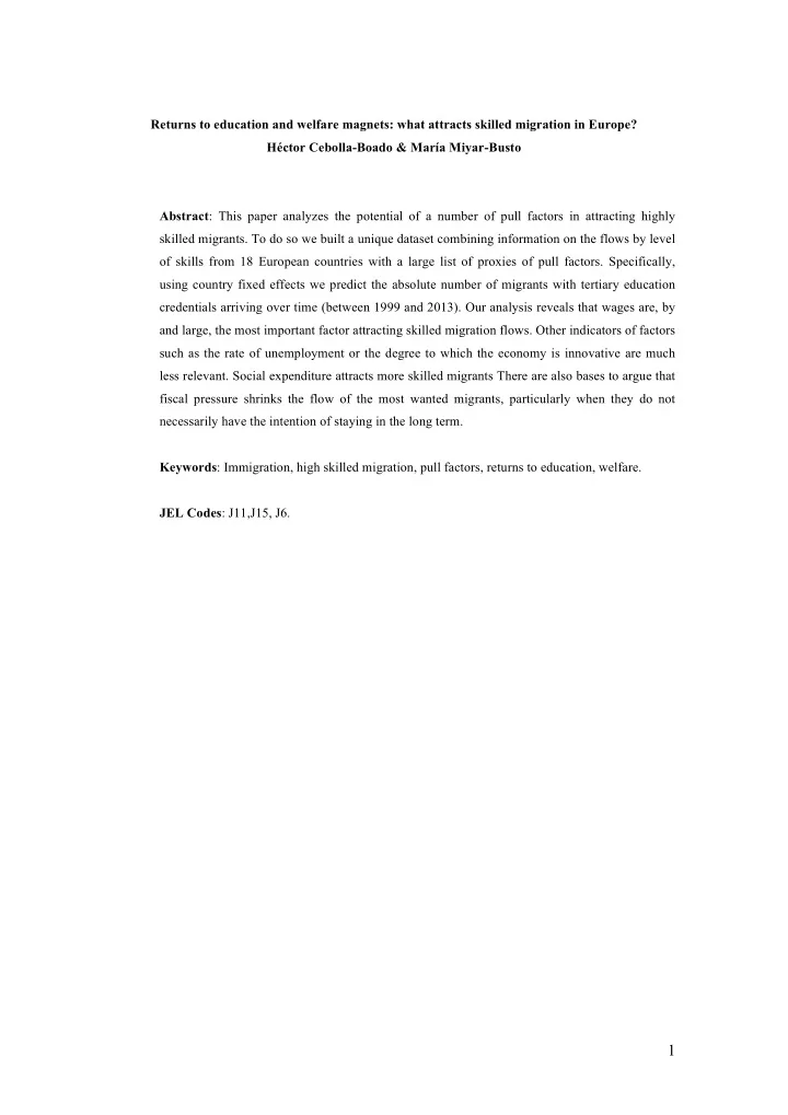
Figure 1. Description of the flow of HSM to selected European countries

Source ELFS and Eurostat statistics. Our calculation

UK NL BE AT NO SE DE FI GR EI DK ES PT LX CY DE NL SE DK PT AT CY BE ES LX FI CH EI NO GR UK SE DE CH LX BE ES DK NL AT FI PT UK CY EI NO GR SE ES NO CH DE EI UK CY NL AT PT FI DK BE GR LX CH BE PT UK DE EI NO LX FI DK CY NL GR AT ES SE IT FI LX SE CH DE ES AT CY PT EI NO UK NL GR BE DK BE UK EI LX IT PT CY AT GR SE FR CH FI NO DE NL DK ES LX ES DK GR NL CH SE FI AT NO DE FR BE EI CY UK IT PT NO UK NL FR CY EI LT DK CH PT ES GR SE LX DE AT IT FI FI UK CH GR IT DK PT ES NL FR LT DE EI AT SE NO CY LX LT NO AT CH ES DE SE FR LX EI IT CY PT BE FI NL DK UK GR SE PT ES LX AT DK UK FR CH CY DE EI NO BE NL LT IT GR BE UK FR LT PT CH CY NO FI DE AT ES GR SE LX NL IT EI DK FR AT UK FI LT CH DK ES NO EI BE DE GR NL IT LX SE

10000 20000 30000 40000

1999200020012002200320042005200620072008200920102011201220132014

Country year Year average

Yrs=0

CY DE NL NO UK ES LX EI GR PT AT UK NL BE AT NO SE DE FI GR EI DK ES PT LX CY DE NL SE DK PT AT CY BE ES LX FI CH EI NO GR UK SE DE CH LX BE ES DK NL AT FI PT UK CY EI NO GR SE ES NO CH DE EI UK CY NL AT PT FI DK BE GR LX CH BE PT UK DE EI NO LX IT FI DK CY NL GR AT ES SE IT FI LX SE CH DE ES AT CY PT EI NO UK NL GR BE DK BE UK EI LX IT PT CY AT GR SE FR CH FI NO DE NL DK ES LX ES DK GR NL CH SE FI AT NO DE FR BE EI CY UK IT PT NO UK NL FR CY EI LT DK CH PT ES GR SE LX DE AT IT FI

20000 40000 60000 80000 100000 120000 140000

1999 2000 2001 2002 2003 2004 2005 2006 2007 2008

Country year Year average

Yrs=5

SLIDE 18

18

Figure 2. Summary of findings for the effect of pull factors on the number of arrivals of highly skilled migrants. Standardized estimates.

Estimates obtained from time series regression models with country fixed effects (models shown in tables A.3 to A.7 in the Appendix).

Wages: 2013 constant prices at 2013 PPPs Prices: Relative consumer price index Unemployment rate: tertiary education Unemp: Less than 1 month Unemp: From 1 to 3 months Unemp: From 3 to 6 months Unemp: From 6 months to 1 year Unemp: More than 1 year GINI Patents: PCT Social Exp: Active labor market prog. Social Exp: Health Social Exp: Social expenditure Taxes: Single 100% av.earnings, no child Female life expectancy

HSM (yrs of residence<0)

• 14000
• 11000
• 8000
• 5000
• 2000

1000 4000 Wages: 2013 constant prices at 2013 PPPs Prices: Relative consumer price index Unemployment rate: tertiary education Unemp: Less than 1 month Unemp: From 1 to 3 months Unemp: From 3 to 6 months Unemp: From 6 months to 1 year Unemp: More than 1 year GINI Patents: PCT Social Exp: Active labor market prog. Social Exp: Health Social Exp: Social expenditure Taxes: Single 100% av.earnings, no child Female life expectancy

HSM (yrs of residence=5)

• 30000
• 20000
• 10000

10000 20000 30000 40000 50000

SLIDE 19

19 Tables

Table 1. Summary of findings. Pull factors on percentage of skilled migrants

Returns to education

Unit

Estimate Welfare magnet

Unit

Estimate

• Av. wage 2013 PPP

NCU/100

Yrs=0

0.32*

Active labor market policies

% GDP

Yrs=0

• 8493.4***

Yrs=5

2.36**

Yrs=5

• 3248.3

Prices Yrs=0 57.0 Health

% GDP

Yrs=0

436.8

Yrs=5

133.4

Yrs=5

13429.5***

Unemp.: tertiary

%

Yrs=0

• 739.8**

Social exp. (overall)

% GDP

Yrs=0

• 1367.9

Yrs=5

• 4176.8**

Yrs=5

36926.5***

Less than 1 month

% male u

Yrs=0

86.9

Single 167% earnings, childless

%

Yrs=0

• 896.7***

Yrs=5

803.7*

Yrs=5

444.7

From 1 to 3 months

% male u

Yrs=0

200.7*

Female life expectancy

Yrs.

Yrs=0

497.6

Yrs=5

621.0

Yrs=5

7626.1***

From 3 to 6 months

% male u

Yrs=0

234.4

Yrs=5

• 113.1

From 6 months to 1 year

% male u

Yrs=0

23.0

Yrs=5

• 339.2

More than 1 year

% male u

Yrs=0

• 160.4**

Yrs=5

• 777.5**

Patents (PCT)

Number

Yrs=0

0.23

GINI

Scale 0-1

Yrs=0

13359.2

Yrs=5

• 287723.2

Legend: NCU: National Currency Units. USD: United States Dollars. Source: Estimates obtained from time series regression models with country fixed effects (models shown in tables A.3 to A.7 in the Appendix). All models control for GDP growth (1 year lag)

SLIDE 20

20

Table 2. Summary of hypotheses, indicators and empirical results (signs and statistical significance). Main argument Indicator Definition N yrs 0 N yrs 5 Returns to education Average wage PPPs + + Prices Relative consumer prices + + Unemployment rate

• Duration of U.

Less than a month + + 1 to 3 months + + 3 to 6 months + + 6 months to 1 year +

• More than a year
• Patents

PCT + + Inequality GINI +

• Welfare magnets

Taxes Single at 167% of average earnings, no child

• +

Social exp. Active labor market programs

• Health

+ + Social expenditure (overall)

• +

Life style Life style Female life expectancy + +

Source: Authors’ elaboration. Shaded areas are statistically significant.

SLIDE 21

21 Appendix Table A.1. Migrants 25-65, with tertiary education and less than 1 year of residence in selected ELFS countries from 1999 to 2013.

Country N FI Finland 78 CY Cyprus 139 DK Denmark 168 GR Greece 184 LU Luxembourg 188 PT Portugal 261 NO Norway 282 IT Italy 345 SE Sweden 347 NL Netherlands 376 AT Austria 593 IE Ireland 630 FR France 1016 BE Belgium 1669 CH Switzerland 1670 ES Spain 1782 UK United Kingdom 2957 DE Germany 8964

Source ELFS. Our calculations.

Table A.2. Summary of the availability of country year information on the arrivals

• f migrants with tertiary education in our dataset

1999 2000 2001 2002 2003 2004 2005 2006 2007 2008 2009 2010 2011 2012 2013 AT x x x x x x x x x x x x x x x BE x x x x x x x x x x x x x x DK x x x x x x x x x x x x x x FI x x x x x x x x x x x x x x FR x x x x x x x x x x x x x x DE x x x x x x x x x x x x x x x GR x x x x x x x x x x x x x x x EI x x x x x x x x x x x x x x x UK x x x x x x x x x x x x x x x CY x x x x x x x x x x x x x x IT x x x x x x x x x x LX x x x x x x x x x x x x x x x NL x x x x x x x x x x x x x x x NO x x x x x x x x x x x x x x x PT x x x x x x x x x x x x x x

SLIDE 22

22

Source: Authors’ elaboration.

Figure A.1. Sample of foreigners arrived in 2007 by time of residence in three selected countries.

Source ELFS. Our calculations.

ES x x x x x x x x x x x x x x x CH x x x x x x x x x x x x x SE x x x x x x x x x x x x x x

SLIDE 23

23 Figure A.2.1 Distribution of arrivals of migrants with tertiary education (aged 25- 65) in selected ELFS countries from 1999 to 2013 (years of residence=0)

Source ELFS, our calculations.

Figure A.2.2 Distribution of arrivals of migrants with tertiary education (aged 25- 65) in selected ELFS countries from 1999 to 2013 (years of residence=5)

10000 20000 30000 40000 10000 20000 30000 40000 10000 20000 30000 40000 10000 20000 30000 40000

2000 2005 2010 2015 2000 2005 2010 2015 2000 2005 2010 2015 2000 2005 2010 2015 2000 2005 2010 2015 AT BE DK FI FR DE GR EI IT LX NL NO PT ES CH SE UK CY

Absolute flow of HSM (years of residence=0)

SLIDE 24

24

Source ELFS. Our calculations.

Table A.3 Returns to education (1) salaries and prices

(1) (2) (3) (4) (5) (6) Yrs=0 Yrs=0 Yrs=0 Yrs=5 Yrs=5 Yrs=5 Average wage 2013 PPP 0.32* 2.36** (0.14) (0.70) Relative consumer prices 57.0 133.4 (60.2) (319.2) Patents (PCT) 0.23 3.65 (0.54) (2.14) Increase in GDP 347.7** 257.0* 233.3* 1061.1 979.4 684.9 (120.9) (113.4) (110.5) (857.6) (942.0) (890.8) Constant

• 3781.3

3730.8 8876.6***

• 63895.1*

16746.0 21820.4*** (5984.8) (6114.8) (1521.0) (28246.3) (33070.9) (5886.9) N 216 216 216 135 135 135 Sigma(u) 8251.8 8472.6 8098.4 37711.2 25665.0 25665.0 Sigma(e) 4418.4 4463.5 4471.5 13607.2 14078.4 14078.4 F 4.73 2.66 2.29 6.14 1.92 1.92 All independent variables are 1 year lagged. Standard errors in parentheses * p<0.05, ** p<0.01, *** p<0.001 Source ELFS and OECD. Our calculations.

Table A.4 Returns to education (2) duration of unemployment

(1) (2) (3) (4) (5) (6) (7) (8) (9) (10) Yrs=0 Yrs=0 Yrs=0 Yrs=0 Yrs=0 Yrs=5 Yrs=5 Yrs=5 Yrs=5 Yrs=5 >1 month 86.9 803.7* (83.3) (366.1) 1-3 months 200.7* 621.0 (87.6) (364.7) 3-6 months 234.4

• 113.1

(133.5) (625.7) 6 months-1 yr 23.0

• 339.2

(118.1) (546.5) > 1 yr

• 160.4**
• 777.5**

(54.0) (285.7) Increase in GDP 249.3* 309.4** 301.1* 256.5* 355.4** 1274.3 1487.5 884.6 912.2 2386.7* (113.4) (114.9) (116.2) (115.8) (116.5) (952.6) (1001.2) (1007.9) (959.9) (1071.2) Constant 8392.8*** 5429.3** 5309.2* 9050.3*** 14655.3*** 19523.8** 16960.7 32850.7** 36563.7*** 52404.7*** (1080.6) (1793.0) (2388.6) (2109.6) (1786.4) (5947.8) (8649.0) (12189.3) (9917.6) (8522.5)

50000 100000 150000 50000 100000 150000 50000 100000 150000 50000 100000 150000

2000 2005 2010 2015 2000 2005 2010 2015 2000 2005 2010 2015 2000 2005 2010 2015 2000 2005 2010 2015 AT BE DK FI FR DE GR EI IT LX NL NO PT ES CH SE UK CY

Absolute flow of HSM (years of residence=5)

SLIDE 25

25

N 211 211 211 211 211 130 130 130 130 130 Sigma(u) 8542.4 8733.0 8629.3 8558.3 8816.4 37255.1 36388.2 35569.4 35562.4 39117.1 Sigma(e) 4499.5 4451.8 4476.4 4511.8 4412.0 14202.8 14321.9 14505.6 14482.6 14046.7 F 3.02 5.15 4.04 2.48 6.98 2.91 1.94 0.50 0.67 4.21 All independent variables are 1 year lagged. Standard errors in parentheses * p<0.05, ** p<0.01, *** p<0.001 Source ELFS and OECD. Our calculations.

SLIDE 26

26 Table A.5 Returns to education (3) inequality and patents

(1) (2) (3) (4) Yrs=0 Yrs=5 Yrs=0 Yrs=5 GINI 13359.2

• 287723.2

(42440.5) (269488.0) Patent (PCT) 0.23 3.65 (0.54) (2.14) Constant 5820.3 120061.6 8876.6*** 21820.4*** (12515.1) (79356.9) (1521.0) (5886.9) Increase in GDP 304.1* 2425.3 233.3* 684.9 (132.7) (2261.0) (110.5) (890.8) N 134 71 216 135 Sigma(u) 9175.6 42251.6 8098.4 25665.0 Sigma(e) 4465.1 17721.0 4471.5 14078.4 F 2.76 1.04 2.29 1.92 All independent variables are 1 year lagged. Standard errors in parentheses * p<0.05, ** p<0.01, *** p<0.001 Source ELFS and OECD. Our calculations.

Table A.6 Welfare magnet (1) public spending as % of GDP

(1) (2) (3) (4) (5) (6) Yrs=0 Yrs=0 Yrs=0 Yrs=5 Yrs=5 Yrs=5 Active labor market policies

• 8493.4***
• 3248.3

(2168.3) (10963.3) Health 436.8 13429.5*** (642.2) (3248.1) Social expenditure (overall)

• 1367.9

36926.5*** (1396.0) (8254.3) Increase in GDP 196.6 279.7* 138.2 1157.5 1793.9 2794.7** (105.4) (135.6) (140.8) (1023.1) (941.6) (985.5) Constant 16197.0*** 6604.6 12920.2*** 7830.5

• 114054.9
• 110936.2

(1761.8) (4173.9) (3577.0) (58897.3) (62073.7) (60133.2) N 200 200 200 125 125 125 Sigma(u) 9190.7 8424.8 8521.2 36925.6 37007.3 56689.8 Sigma(e) 4067.3 4230.8 4225.0 13948.8 12940.9 12789.0 F 9.96 2.35 2.60 0.64 6.41 7.40 All independent variables are 1 year lagged. Standard errors in parentheses * p<0.05, ** p<0.01, *** p<0.001 Source ELFS and OECD. Our calculations.

Table A.7 Welfare magnet (2) public spending as % of GDP

(1) (2) (3) (4) Yrs=0 Yrs=5 Yrs=0 Yrs=5 Single at 167%

• 896.7***

444.7 (243.4) (1282.4) Female life expectancy 497.6 7626.1*** (378.7) (1768.7) Increase in GDP 321.7** 1216.4 311.4* 770.8 (113.0) (999.4) (125.6) (832.2) Constant 50477.5*** 9397.8

• 31667.4
• 593509.7***

(11123.1) (58406.4) (31340.1) (144756.3) N 206 125 216 135 Sigma(u) 9657.7 36827.7 8528.6 34589.9 Sigma(e) 4364.4 13888.7 4454.1 13232.8 F 9.74 0.93 3.08 9.83 All independent variables are 1 year lagged. Standard errors in parentheses * p<0.05, ** p<0.01, *** p<0.001 Source ELFS and OECD. Our calculations.