1 Alternative File Organizations Model for Analyzing Access Costs - - PDF document

SLIDE 1

1

Database Internals

Zachary Ives CSE 594 Spring 2002

Some slide contents by Raghu Ramakrishnan

2

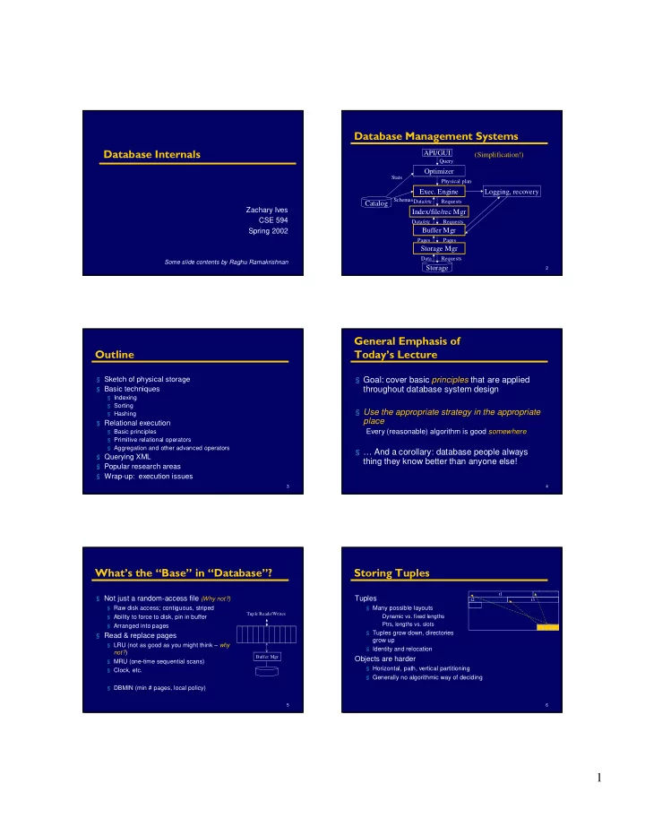
Database Management Systems

API/GUI Optimizer Storage Mgr

• Exec. Engine

Storage Catalog

Query Physical plan Pages Requests Data Pages Stats Schemas

(Simplification!) Buffer Mgr Index/file/rec Mgr

Data/etc Requests Requests Data/etc

Logging, recovery

3

Outline

§ Sketch of physical storage § Basic techniques

§ Indexing § Sorting § Hashing

§ Relational execution

§ Basic principles § Primitive relational operators § Aggregation and other advanced operators

§ Querying XML § Popular research areas § Wrap-up: execution issues

4

General Emphasis of Today’s Lecture

§ Goal: cover basic principles that are applied throughout database system design § Use the appropriate strategy in the appropriate place

Every (reasonable) algorithm is good somewhere

§ … And a corollary: database people always thing they know better than anyone else!

5

What’s the “Base” in “Database”?

§ Not just a random-access file (Why not?)

§ Raw disk access; contiguous, striped § Ability to force to disk, pin in buffer § Arranged into pages

§ Read & replace pages

§ LRU (not as good as you might think – why not?) § MRU (one-time sequential scans) § Clock, etc. § DBMIN (min # pages, local policy)

Buffer Mgr Tuple Reads/Writes 6

Storing Tuples

Tuples

§ Many possible layouts Dynamic vs. fixed lengths Ptrs, lengths vs. slots § Tuples grow down, directories grow up § Identity and relocation

Objects are harder

§ Horizontal, path, vertical partitioning § Generally no algorithmic way of deciding

t1 t2 t3

SLIDE 2

2

Alternative File Organizations

Many alternatives, each ideal for some situation, and poor for others:

§ Heap files: for full file scans or frequent updates

Data unordered Write new data at end

§ Sorted Files: if retrieved in sort order or want range

Need external sort or an index to keep sorted

§ Hashed Files: if selection on equality Collection of buckets with primary & overflow pages Hashing function over search key attributes

Model for Analyzing Access Costs

We ignore CPU costs, for simplicity:

§ b(T): The number of data pages in table T § r(T): Number of records in table T § D: (Average) time to read or write disk page § Measuring number of page I/O’s ignores gains of pre-fetching blocks of pages; thus, I/O cost is only approximated. § Average-case analysis; based on several simplistic assumptions. * Good enough to show the overall trends!

Assumptions in Our Analysis

§ Single record insert and delete. § Heap Files:

§ Equality selection on key; exactly one match. § Insert always at end of file.

§ Sorted Files:

§ Files compacted after deletions. § Selections on sort field(s).

§ Hashed Files:

§ No overflow buckets, 80% page occupancy.

Cost of Operations

Delete Insert Range Search Equality Search Scan all recs Hashed File Sorted File Heap File

11

* Several assumptions underlie these (rough) estimates!

2D Search + b(T) D Search + D Delete 2D Search + b(T) D 2D Insert 1.25 b(T) D D log2 b(T) + (# pages with matches) b(T) D Range Search D D log2 b(T) b(T) D / 2 Equality Search 1.25 b(T) D b(T)D b(T) D Scan all recs Hashed File Sorted File Heap File

Cost of Operations

12

Speeding Operations over Data

§ Three general data organization techniques:

§ Indexing § Sorting § Hashing

SLIDE 3

3

Technique I: Indexing

§ An index on a file speeds up selections on the search key attributes for the index (trade space for speed).

§ Any subset of the fields of a relation can be the search key for an index on the relation. § Search key is not the same as key (minimal set of fields that uniquely identify a record in a relation).

§ An index contains a collection of data entries, and supports efficient retrieval of all data entries k* with a given key value k.

GMUW §4.1-4.3

Alternatives for Data Entry k* in Index

§ Three alternatives:

Data record with key value k

Clustered -> fast lookup

8 Index is large; only 1 can exist

` <k, rid of data record with search key value k>, OR ´ <k, list of rids of data records with search key k>

Can have secondary indices Smaller index may mean faster lookup

8 Often not clustered -> more expensive to use

§ Choice of alternative for data entries is

• rthogonal to the indexing technique used to

locate data entries with a given key value k.

Classes of Indices

§ Primary vs. secondary: primary has primary key § Clustered vs. unclustered: order of records and index approximately same

§ Alternative 1 implies clustered, but not vice-versa. § A file can be clustered on at most one search key.

§ Dense vs. Sparse: dense has index entry per data value; sparse may “skip” some

§ Alternative 1 always leads to dense index. § Every sparse index is clustered! § Sparse indexes are smaller; however, some useful

• ptimizations are based on dense indexes.

Clustered vs. Unclustered Index

Suppose Index Alternative (2) used, records are stored in Heap file

§ Perhaps initially sort data file, leave some gaps § Inserts may require overflow pages

Index entries Data entries direct search for (Index File) (Data file) Data Records data entries Data entries Data Records CLUSTERED UNCLUSTERED

B+ Tree: The World’s Favourite Index

§ Insert/delete at log F N cost

§ (F = fanout, N = # leaf pages) § Keep tree height-balanced

§ Minimum 50% occupancy (except for root). § Each node contains d <= m <= 2d entries. d is called the order of the tree. § Supports equality and range searches efficiently.

Index Entries Data Entries ("Sequence set") (Direct search)

Example B+ Tree

§ Search begins at root, and key comparisons direct it to a leaf. § Search for 5*, 15*, all data entries >= 24* ...

* Based on the search for 15*, we know it is not in the tree!

Root 17 24 30 2* 3* 5* 7* 14* 16* 19* 20* 22* 24* 27* 29* 33* 34* 38* 39* 13

SLIDE 4

4

B+ Trees in Practice

§ Typical order: 100. Typical fill-factor: 67%.

§ average fanout = 133

§ Typical capacities:

§ Height 4: 1334 = 312,900,700 records § Height 3: 1333 = 2,352,637 records

§ Can often hold top levels in buffer pool:

§ Level 1 = 1 page = 8 Kbytes § Level 2 = 133 pages = 1 Mbyte § Level 3 = 17,689 pages = 133 MBytes

Inserting Data into a B+ Tree

§ Find correct leaf L. § Put data entry onto L.

§ If L has enough space, done! § Else, must split L (into L and a new node L2) Redistribute entries evenly, copy up middle key. Insert index entry pointing to L2 into parent of L.

§ This can happen recursively

§ To split index node, redistribute entries evenly, but push up middle key. (Contrast with leaf splits.)

§ Splits “grow” tree; root split increases height.

§ Tree growth: gets wider or one level taller at top.

Inserting 8* into Example B+ Tree

§ Observe how minimum occupancy is guaranteed in both leaf and index pg splits. § Recall that all data items are in leaves, and partition values for keys are in intermediate nodes

Note difference between copy-up and push-up.

22

Inserting 8* Example: Copy up

Root 17 24 30 2* 3* 5* 7* 14* 16* 19* 20* 22* 24* 27* 29* 33* 34* 38* 39* 13

Want to insert here; no room, so split & copy up:

2* 3* 5* 7* 8* 5 Entry to be inserted in parent node. (Note that 5 is continues to appear in the leaf.) s copied up and 8* 23

Inserting 8* Example: Push up

Root 17 24 30 2* 3* 14* 16* 19* 20* 22* 24* 27* 29* 33* 34* 38* 39* 13 5* 7* 8* 5

Need to split node & push up

5 24 30 17 13 Entry to be inserted in parent node. (Note that 17 is pushed up and only appears once in the index. Contrast this with a leaf split.)

Deleting Data from a B+ Tree

§ Start at root, find leaf L where entry belongs. § Remove the entry.

§ If L is at least half-full, done! § If L has only d-1 entries, Try to re-distribute, borrowing from sibling (adjacent node with same parent as L). If re-distribution fails, merge L and sibling.

§ If merge occurred, must delete entry (pointing to L or sibling) from parent of L. § Merge could propagate to root, decreasing height.

SLIDE 5

5

B+ Tree Summary

B+ tree and other indices ideal for range searches, good for equality searches.

§ Inserts/deletes leave tree height-balanced; logF N cost. § High fanout (F) means depth rarely more than 3 or 4. § Almost always better than maintaining a sorted file. § Typically, 67% occupancy on average. § Note: Order (d) concept replaced by physical space criterion in practice (“at least half-full”). Records may be variable sized Index pages typically hold more entries than leaves

26

Other Kinds of Indices

§ Multidimensional indices

§ R-trees, kD-trees, …

§ Text indices

§ Inverted indices

§ etc.

27

Objects and Indices

Multi-level hierarchy: Object.Subobject.Subsubobject

§ Want to query for objects with submember of specific value § Vehicles with Vehicle.Mfr.Name = “Ferrari” § Companies with Company.Division.Loc = “Modena”

360 Modena 03 10 TT 04 02 Testarosa 03 01 05, 06 Ferrari 03 Modena Assembly 05 Vehicle(Mfr, Model) Division(Name, Loc) Modena Design 06 Company(Name, Division)

28

360 Modena 03 10 Z3 04 02 Testarosa 03 01 05, 06 Ferrari 03 Modena Assembly 05 Vehicle(Mfr, Model) Modena Design 06 Company(Name, Division) 07 BMW 04 Modena Quality Ctrl. 07

Example Class Hierarchy

Division(Name, Loc)

29

Access Support Relations

§ Speed up finding a sub- or super-object § Create a table with a tuple per path through the object hierarchy VehicleOID CompanyOID DivisionOID

30

Beyond Objects

More complex than objects: semistructured data (e.g. XML)

§ Self-describing (embedded labels) § Irregular structure § “Weaker” typing (potentially) § XPath expressions

OO indexing techniques applicable? Why or why not?

SLIDE 6

6

31

Speeding Operations over Data

§ Three general data organization techniques:

§ Indexing § Sorting § Hashing

Technique II: Sorting

§ Pass 1: Read a page, sort it, write it.

§ only one buffer page is used

§ Pass 2, 3, …, etc.:

§ three buffer pages used.

Main memory buffers

INPUT 1 INPUT 2 OUTPUT

Disk Disk GMUW §2.3

Two-Way External Merge Sort

§ Each pass we read, write each page in file. § N pages in the file => the number of passes § Total cost is: § Idea: Divide and conquer: sort subfiles and merge   = + log2 1 N

 

( )

2 1

2

N N log +

Input file 1-page runs 2-page runs 4-page runs 8-page runs PASS 0 PASS 1 PASS 2 PASS 3 9 3,4 6,2 9,4 8,7 5,6 3,1 2 3,4 5,6 2,6 4,9 7,8 1,3 2 2,3 4,6 4,7 8,9 1,3 5,6 2 2,3 4,4 6,7 8,9 1,2 3,5 6 1,2 2,3 3,4 4,5 6,6 7,8

General External Merge Sort

§ To sort a file with N pages using B buffer pages:

§ Pass 0: use B buffer pages. Produce sorted runs of B pages each. § Pass 2, …, etc.: merge B-1 runs.

  N B /

B Main memory buffers

INPUT 1 INPUT B-1 OUTPUT

Disk Disk

INPUT 2

. . . . . . . . .

* How can we utilize more than 3 buffer pages?

Cost of External Merge Sort

§ Number of passes: § Cost = 2N * (# of passes) § With 5 buffer pages, to sort 108 page file:

§ Pass 0: = 22 sorted runs of 5 pages each (last run is only 3 pages) § Pass 1: = 6 sorted runs of 20 pages each (last run is only 8 pages) § Pass 2: 2 sorted runs, 80 pages and 28 pages § Pass 3: Sorted file of 108 pages

   

B N

B

/ log 1

1 −

+

  108 5 /   22 4 /

36

Speeding Operations over Data

§ Three general data organization techniques:

§ Indexing § Sorting § Hashing

SLIDE 7

7

37

Technique 3: Hashing

§ A familiar idea:

§ Requires “good” hash function (may depend on data) § Distribute data across buckets § Often multiple items in same bucket (buckets might overflow)

§ Types of hash tables:

§ Static § Extendible (requires directory to buckets; can split) § Linear (two levels, rotate through + split; bad with skew) § Can be the basis of disk-based indices! We won’t get into detail because of time, but see text GMUW §4.4

38

Making Use of the Data + Indices: Query Execution

§ Query plans & exec strategies § Basic principles § Standard relational operators § Querying XML

GMUW §6

39

Query Plans

§ Data-flow graph of relational algebra

• perators

§ Typically: determined by

• ptimizer

Select

Client = “Atkins”

Join

PressRel.Symbol = Clients.Symbol

Scan

PressRel

Scan

Clients

Join

Symbol = Northwest.CoSymbol

Project

CoSymbol

Scan

Northwest

SELECT * FROM PressRel p, Clients C WHERE p.Symbol = c.Symbol AND c.Client = ‘Atkins’ AND c.Symbol IN (SELECT CoSymbol FROM Northwest)

40

Execution Strategy Issues

§ Granularity & parallelism:

§ Pipelining vs. blocking § Materialization

Select

Client = “Atkins”

Join

PressRel.Symbol = Clients.Symbol

Scan

PressRel

Scan

Clients

Join

Symbol = Northwest.CoSymbol

Project

CoSymbol

Scan

Northwest 41

Iterator-Based Query Execution

§ Execution begins at root

§ open, next, close § Propagate calls to children

May call multiple child nexts

! Efficient scheduling & resource usage

Can you think of alternatives and their benefits?

Select

Client = “Atkins”

Join

PressRel.Symbol = Clients.Symbol

Scan

PressRel

Scan

Clients

Join

Symbol = Northwest.CoSymbol

Project

CoSymbol

Scan

Northwest 42

Basic Principles

§ Many DB operations require reading tuples, tuple vs. previous tuples, or tuples vs. tuples in another table § Techniques generally used:

§ Iteration: for/while loop comparing with all tuples on disk § Index: if comparison of attribute that’s indexed, look up matches in index & return those § Sort: iteration against presorted data (interesting orders) § Hash: build hash table of the tuple list, probe the hash table

* Must be able to support larger-than-memory data

SLIDE 8

8

43

Basic Operators

§ One-pass operators:

§ Scan § Select § Project

§ Multi-pass operators:

§ Join

Various implementations Handling of larger-than-memory sources

§ Semi-join § Aggregation, union, etc.

44

1-Pass Operators: Scanning a Table

§ Sequential scan: read through blocks of table § Index scan: retrieve tuples in index order

§ May require 1 seek per tuple! § Cost in page reads -- b(T) blocks, r(T) tuples

§ b(T) pages for sequential scan § Up to r(T) for index scan if unclustered index § Requires memory for one block

45

1-Pass Operators: Select (σ σ σ σ)

§ Typically done while scanning a file § If unsorted & no index, check against predicate:

Read tuple While tuple doesn’t meet predicate Read tuple Return tuple

§ Sorted data: can stop after particular value encountered § Indexed data: apply predicate to index, if possible § If predicate is:

§ conjunction: may use indexes and/or scanning loop above (may need to sort/hash to compute intersection) § disjunction: may use union of index results, or scanning loop

46

1-Pass Operators: Project (Π Π Π Π)

§ Simple scanning method often used if no index:

Read tuple While more tuples Output specified attributes Read tuple

§ Duplicate removal may be necessary

§ Partition output into separate files by bucket, do duplicate removal on those § If have many duplicates, sorting may be better

§ If attributes belong to an index, don’t need to retrieve tuples!

47

Multi-pass Operators: Join (!" !" !" !") -- Nested-Loops Join

§ Requires two nested loops:

For each tuple in outer relation For each tuple in inner, compare If match on join attribute, output

§ Results have order of outer relation § Can do over indices ! Very simple to implement, supports any joins predicates ! Supports any join predicates " Cost: # comparisons = t(R) t(S) # disk accesses = b(R) + t(R) b(S) Join

• uter

inner

48

Block Nested-Loops Join

§ Join a page (block) at a time from each table:

For each page in outer relation For each page in inner, join both pages If match on join attribute, output

! More efficient than previous approach: " Cost: # comparisons still = t(R) t(S) # disk accesses = b(R) + b(R) * b(S)

SLIDE 9

9

49

Index Nested-Loops Join

For each tuple in outer relation For each match in inner’s index Retrieve inner tuple + output joined tuple

§ Cost: b(R) + t(R) * cost of matching in S § For each R tuple, costs of probing index are about:

§ 1.2 for hash index, 2-4 for B+-tree and: Clustered index: 1 I/O on average Unclustered index: Up to 1 I/O per S tuple

50

Two-Pass Algorithms

Sort-based

Need to do a multiway sort first (or have an index) Approximately linear in practice, 2 b(T) for table T

Hash-based

Store one relation in a hash table

51

(Sort-)Merge Join

§ Requires data sorted by join attributes

Merge and join sorted files, reading sequentially a block at a time

§ Maintain two file pointers

While tuple at R < tuple at S, advance R (and vice versa) While tuples match, output all possible pairings

§ Preserves sorted order of “outer” relation ! Very efficient for presorted data ! Can be “hybridized” with NL Join for range joins " May require a sort before (adds cost + delay) § Cost: b(R) + b(S) plus sort costs, if necessary In practice, approximately linear, 3 (b(R) + b(S))

52

Hash-Based Joins

§ Allows partial pipelining of operations with equality comparisons § Sort-based operations block, but allow range and inequality comparisons § Hash joins usually done with static number of hash buckets

§ Generally have fairly long chains at each bucket § What happens when memory is too small?

53

Hash Join

Read entire inner relation into hash table (join attributes as key) For each tuple from

• uter, look up in hash

table & join

! Very efficient, very good for databases " Not fully pipelined " Supports equijoins

• nly

" Delay-sensitive

tuple tuple tuple 54

Running out of Memory

§ Prevention: First partition the data by value into memory-sized groups

Partition both relations in the same way, write to files Recursively join the partitions

§ Resolution: Similar, but do when hash tables full

Split hash table into files along bucket boundaries Partition remaining data in same way Recursively join partitions with diff. hash fn!

§ Hybrid hash join: flush “lazily” a few buckets at a time § Cost: <= 3 * (b(R) + b(S))

SLIDE 10

10

55

Pipelined Hash Join Useful for Joining Web Sources

§ Two hash tables § As a tuple comes in, add to the appropriate side & join with

• pposite table

! Fully pipelined, adaptive to source data rates ! Can handle overflow as with hash join " Needs more memory

tuple tuple tuple 56

The Semi-Join/Dependent Join

§ Take attributes from left and feed to the right source as input/filter § Important in data integration § Simple method:

for each tuple from left send to right source get data back, join

§ More complex:

§ Hash “cache” of attributes & mappings § Don’t send attribute already seen § Bloom joins (use bit-vectors to reduce traffic)

JoinA.x = B.y A B

x

57

Aggregation (γ γ γ γ)

§ Need to store entire table, coalesce groups with matching GROUP BY attributes § Compute aggregate function over group:

§ If groups are sorted or indexed, can iterate:

Read tuples while attributes match, compute aggregate At end of each group, output result

§ Hash approach:

Group together in hash table (leave space for agg values!) Compute aggregates incrementally or at end At end, return answers

§ Cost: b(t) pages. How much memory?

58

Other Operators

§ Duplicate removal very similar to grouping

§ All attributes must match § No aggregate

§ Union, difference, intersection:

§ Read table R, build hash/search tree § Read table S, add/discard tuples as required § Cost: b(R) + b(S)

59

Relational Operations

In a whirlwind, you’ve seen most of relational

• perators:

§ Select, Project, Join § Group/aggregate § Union, Difference, Intersection § Others are used sometimes:

Various methods of “for all,” “not exists,” etc Recursive queries/fixpoint operator etc.

60

Recall XML

<db> <store> <manager>Griffith</manager> <manager>Sims</manager> <location> <address>12 Pike Pl.</address> <city>Seattle</city> </location> </store> <store> <manager>Jones</manager> <address>30 Main St.</address> <city>Berkeley</city> </store> </db>

Element Data value

SLIDE 11

11

61

Querying XML with XQuery

“Query over all stores, managers, and cities”: Query operations evaluated over all possible tuples

• f ($s, $m, $c) that can be matched on input

FOR $s = (document)/db/store, $m = $s/manager/data(), $c = $s//city/data() WHERE {join + select conditions} RETURN {XML output}

62

Processing XML

§ Bind variables to subtrees; treat each set of bindings as a tuple § Select, project, join, etc. on tuples of bindings § Plus we need some new operators:

§ XML construction:

Create element (add tags around data) Add attribute(s) to element (similar to join) Nest element under other element (similar to join)

§ Path expression evaluation – create the binding tuples

63

Standard Method: XML Query Processing in Action

Parse XML:

<db> <store> <manager>Griffith</manager> <manager>Sims</manager> <location> <address>12 Pike Pl.</address> <city>Seattle</city> </location> </store> …

Match paths:

$s = (root)/db/store $m = $s/manager/data() $c = $s//city/data() $s $m $c #1 Griffith Seattle #1 Sims Seattle #2 Jones Madison

db store store Griffith Seattle manager city Jones 30 Main St. manager address location 12 Pike Pl. address city Madison manager Sims db store store Griffith Seattle manager city Jones 30 Main St. manager address location 12 Pike Pl. address city Madison #1 #2 manager Sims

64

X-Scan: “Scan” for Streaming XML

§ We often re-read XML from net on every query

Data integration, data exchange, reading from Web

§ Previous systems:

§ Store XML on disk, then index & query § Cannot amortize storage costs

§ X-scan works on streaming XML data

§ Read & parse § Evaluate path expressions to select nodes § Also has support for mapping XML to graphs

65

$s $m $c

X-Scan: Incremental Parsing & Path Matching

</location> </store> <store> <manager>Jones</manager> <address>30 Main St.</address> <city>Berkeley</city> </store> </db> <db> <store> <manager>Griffith</manager> <manager>Sims</manager> <location> <address>12 Pike Pl.</address> <city>Seattle</city> #1 Griffith #1 Sims Seattle Seattle #2 Jones Berkeley #1 #2

Tuples for query:

$s $m $c

1 2 3

db store

4 5 6

manager data()

6 7 8

city data()

66

X-Scan works on Graphs

§ XML allows IDREF-style links within a document

§ Keep track of every ID § Build an “index” of the XML document’s structure; add real edges for every subelement and IDREF § When IDREF encountered, see if ID is known

If so, dereference and follow it Otherwise, parse and index until we get to it, then process the newly indexed data node3 node4 node2 ref=“node4” ref=“node2”

SLIDE 12

12

67

Building XML Output

§ Need the following operations:

§ Create XML Element § Create XML Attribute § Output Value/Variable into XML content § Nest XML subquery results into XML element

(Looks very much like a join between parent query and subquery!)

68

An XML Query

§ X-scan creates tuples § Select, join as usual § Construct results

§ Output variable § Create element around content

§ A few key extensions to standard models!

X-scan X-scan

$b = db/book $pID = $b/@publisher $t = $b/title, $ed = $b/editors/name $p = db/company $pID2 = $p/@ID

books.xml pubs.xml

$pID = $pID2

Output Element Output Element Element

$t <name>, 1 $p <publisher>,1 <book>,2 b pID t ed p pID2 b pID t ed p pID2 b pID t ed p pID2 publisher name b pID t ed p pID2 b pID t ed p pID2 name b pID t ed p pID2 name publisher name book b pID t ed $ed = "Stonebraker" b pID t ed p pID2

69

Where’s Query Execution Headed?

§ Adaptive scheduling of operations – adjusting work to prioritize certain tuples § Robust – as in distributed systems, exploit replicas, handle failures § Show and update partial/tentative results § More interactive and responsive to user § More complex data models –XML, semistructured data

70

Leading into Next Week’s Topic: Execution Issues for the Optimizer

§ Goal: minimize I/O costs! § Try different orders of applying operations

Selectivity estimates

§ Choose different algorithms

§ “Interesting orders” – exploit sorts § Equijoin or range join? § Exploit indices

§ How much memory do I have and need?