1 Problem with Brute force Nave Bayes ( ) ( ) ( ) It cannot - - PDF document

SLIDE 1

1

Discrete Bayesian classifiers

Lecture 5

Outline

Bayes theorem Maximum likelihood classification “Brute force” Bayesian learning Naïve Bayes Bayesian Belief Networks

Bayes theorem

P(c) – prior probability of class c

Expected proportion of data from class c on test

P(x) – prior probability of instance x

Probability of instance with attribute vector x to occur

P(c|x) – probability of an instance being of class c

given it is described by vector of attributes x

P(x|c) – probability of an instance of having

attributes described by x given it comes from class c

( ) ( ) ( ) ( )

x P c P c x P x c P | | =

Maximum likelihood

From training data estimate for all x and ci

P(ci) P(x|ci)

During classification:

Choose class ci with maximal P(ci|x)

P(ci|x) is also called likelihood

‘Brute force’ Bayesian learning

Instance x described by attributes < a1,…,an> Most probable class:

( ) ( ) ( ) ( ) ( ) ( ) ( )

i i n c n i i n c n i c

c P c a a P a a P c P c a a P a a c P x c

i i i

| ,..., max arg ,..., | ,..., max arg ,..., | max arg

1 1 1 1

= = = = =

Example

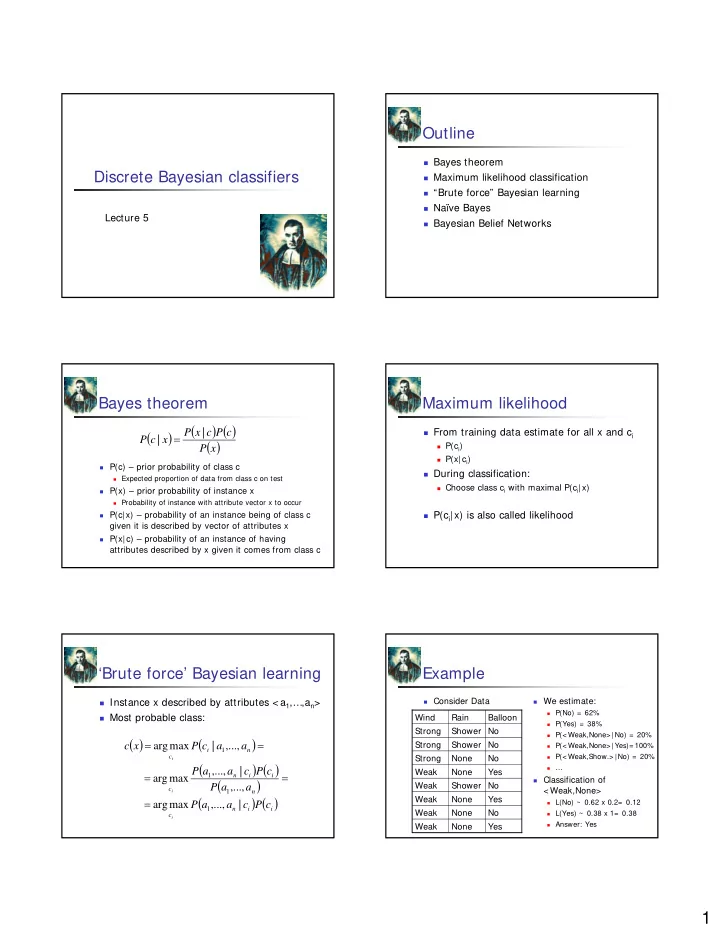
Consider Data We estimate:

P(No) = 62% P(Yes) = 38% P(< Weak,None> |No) = 20% P(< Weak,None> |Yes)= 100% P(< Weak,Show.> |No) = 20% …

Classification of

< Weak,None>

L(No) ~ 0.62 x 0.2= 0.12 L(Yes) ~ 0.38 x 1= 0.38 Answer: Yes

Yes None Weak No None Weak Yes None Weak No Shower Weak Yes None Weak No None Strong No Shower Strong No Shower Strong Balloon Rain Wind

SLIDE 2

2

Problem with ‘Brute force’

It cannot generalize to unseen examples xnew,

because it does not have estimates P(ci|xnew)

It is useless Brute force does not have any bias So in order to make learning possible we

have to introduce a bias

Naïve Bayes

Brute force: Naïve Bayes assumes that attributes are

independent for instances from a given class:

Which gives:

Assumption of independence is often violated

by Naïve Bayes works surprisingly well anyway

( ) ( ) ( )

i i n c

c P c a a P x c

i

| ,..., max arg

1

=

( )

( )

∏

=

j i j i n

c a P c a a P | | ,...,

1

( ) ( )

( )

∏

=

j i j i c

c a P c P x c

i

| max arg

Example

Recall ‘advanced ballooning’ set: Classify: x= < Cloudy, Hot, Shower, Strong>

P(Y|x) ~ P(Y) P(Cl|Y) P(H|Y) P(Sh|Y) P (St|Y)

= 0.5 x 0.5 x 0 x 0.5 x 0.5 = 0

P(N|x) ~ 0.5 x 0.5 x 0.5 x 1 x 1 = 0.125

No Strong Shower Hot Sunny No Strong Shower Cold Cloudy Yes Weak Shower Cold Cloudy Yes Strong None Cold Sunny Fly Balloon Wind Rain Temper. Sky

Missing estimates

What if none of training instances of class ci

have attribute value aj? Then:

P(aj|ci) = 0, and

• no matter what are the values of other attributes

For example:

x = < Sunny, Hot, None, Weak> P(Hot|Yes) = 0, hence P(Yes|x) = 0

( )

( )

| | ,...,

1

= =∏

j i j i n

c a P c a a P

Solution

Let m denote the number of possible values of

attribute aj

For each class let us consider adding m “virtual

examples” with different values of aj

Bayesian estimate for P(aj|ci) becomes: Where:

nci – number of training examples with class ci nciaj – number of training examples with class ci and

attribute aj

( )

m n n c a P

ci ciaj i j

+ + = 1 |

Learning to classify text

For example: is an e-mail a spam? Represent each document by a set of words

Independence assumptions:

Order of words does not matter Co-occurrences of words do not matter

Learning: estimate from training documents:

For every class ci estimate P(ci) For every word w and class ci estimate P(w|ci)

Classification: maximum likelihood

SLIDE 3

3

Learning in detail

Vocabulary = all distinct words in training text For each class ci

• Textci = concatenated documents of class ci

nci = total # words in Textci (count duplicates multiple times) For each word wj in Vocabulary

nciwj = number of times word wj occurred in text Textci (

)

Vocabulary n n c w P

ci ciwj i j

+ + = 1 |

( )

documents

• f

number Total c class

• f

documents

• f

Number c P

i i =

Classification in detail

Index all words in document to classify by j

i.e. denote jth word in the document by wj

Classify: In practice P(wj|ci) are small so their product

is very close to 0; it is better to use: ( )

( )

∏

=

j i j i c

c w P c P document c

i

| max arg ) (

( )

( )

( )

( )⎥

⎦ ⎤ ⎢ ⎣ ⎡ + = = ⎥ ⎦ ⎤ ⎢ ⎣ ⎡ =

∑ ∏

j i j i c j i j i c

c w P c P c w P c P document c

i i

| log log max arg | log max arg ) (

Pre-processing

Allows adding background knowledge May dramatically increase accuracy Sample techniques:

Lemmatisation - converts words to basic form Stop-list - removes 100 most frequent words

Understanding Naïve Bayes

Although Naïve Bayes is considered to be

subsymbolic, the estimated probabilities may give insight on the classification process

For example in spam filtering

Words with maximum P(wj|spam) are the words

whose presence most predicts en e-mail to be a spam e-mail

Bayesian Belief Networks

Naïve Bayes assumption of conditional

independence of attributes is too restrictive for some problems

But some assumptions need to be made to

allow generalization

Bayesian Belief Networks assume conditional

independence among subset of attributes

Allows combining prior knowledge about

(in)dependencies among attributes

Conditional independence

X is conditionally independent of Y given Z if

∀x,y,z: P(X= x | Y= y, Z= z) = P(X= x | Z= z) Usually written: P(X|Y,Z) = P(X|Z) Example:

P(Thunder|Rain,Ligthining)= P(Thunder|Lightning)

Used by Naïve Bayes:

P(A1,A2|C) = P(A1|A2,C) P(A2|C) = P(A1|C)P(A2|C)

Always true Only true if A1 and A2 conditionally independent

SLIDE 4

4

Bayesian Belief Network

Connections describe dependence & causality

Each node is conditionally independent of its

nondescendants, given its immediate predecessors

Examples:

feVer and Headache are independent given flu feVer and weakness are not independent given flu

Headache feVer Weakness Flu

Learning Bayesian Network

Probabilities of attribute values given parents

can be estimated from the training set

Headache feVer Weakness Flu 0.9 0.4 ¬H 0.1 0.6 H ¬F F 0.9 0.2 ¬V 0.1 0.8 V ¬F F 0.95 0.5 0.2 0.1 ¬W 0.05 0.5 0.8 0.9 W ¬F ¬V F¬V ¬FV FV 0.9 ¬F 0.1 F

Inference

During Bayesian classification we compute: In general in Bayesian network with nodes Yi:

Thus

Example: Classify patient: W,V,¬H

P(W,V,¬H,F) = P(W|VF) P(V|F) P(¬H|F) P(F)

( ) ( ) ( ) ( )

i n c i i n c

c a a P c P c a a P x c

i i

, ,..., max arg | ,..., max arg

1 1

= =

( ) ( ) ( )

∏

=

=

n i i i n

Y Parents y P y y P

1 1

| ,...,

( ) ( ) ( ) ( )

c P A Parents a P c a a P

n i i i n

∏

=

=

1 1

| , ,...,

Naïve Bayes network

In case of this network: Headache feVer Sore throat Flu

( ) ( ) ( ) ( ) ( ) ( )

c P c a P c P A Parents a P c a a P

n i i n i i i n

∏ ∏

= =

= =

1 1 1

| | , ,...,

Extensions to Bayesian nets

Network with hidden states, e.g. Learning structure of the network from data

Summary

Inductive bias of Naïve Bayes:

Attributes are independent.

Although this assumption is often violated, it

provides a very efficient tool often used

E.g. For spam filtering.

Applicable to data:

with many attributes (possibly missing), which take discrete values (e.g. words).

Bayesian belief networks

Allow prior knowledge about dependencies