1 Heuristic (Bound- -Guided) Search Guided) Search Bucket Tree - - PDF document

1

On On-

• demand Bound Computation

demand Bound Computation for Finding Leading Solutions for Finding Leading Solutions to Soft Constraints to Soft Constraints

Martin Sachenbacher and Brian C. Williams MIT Computer Science and AI Laboratory September 27, 2004

Finding Finding Leading Solutions Leading Solutions

Many AI problems = Constraint optimization problems

– Diagnosis (state estimation) – Planning – …

Practical AI requirement: Robustness ⇒

Generate solutions in best-first order, until halted

– Most likely diagnoses, until failure is found – Least cost plans, until actions are executable – …

Problem: Not known in advance when halted ⇒

Must generate each solution as quickly as possible

Example: Full Adder Diagnosis Example: Full Adder Diagnosis

Variables {u, v, w, y, a1, a2, e1, e2, o1} {a1, a2, e1, e2, o1} describe modes of gates Gates are either in good (“G”) or broken (“B”) mode

Example: Full Adder Diagnosis Example: Full Adder Diagnosis

And-gates broken with 1% probability Or-, Xor-gates broken with 5% probability Probabilistic valuation structure ([0,1], ≤, *, 1, 0)

Modeling the Example as Soft CSP Modeling the Example as Soft CSP

• 1 v w

G 0 0 B 0 0 B 0 1 B 1 0 B 1 1 .95 .05 .05 .05 .05 e2 u G 0 B 0 B 1 .95 .05 .05 a1 w y G 0 0 G 1 1 B 0 0 B 0 1 B 1 0 B 1 1 .99 .99 .01 .01 .01 .01 a2 u v G 0 0 G 1 1 B 0 0 B 0 1 B 1 0 B 1 1 .99 .99 .01 .01 .01 .01 e1 u y G 1 0 G 0 1 B 0 0 B 0 1 B 1 0 B 1 1 .95 .95 .05 .05 .05 .05

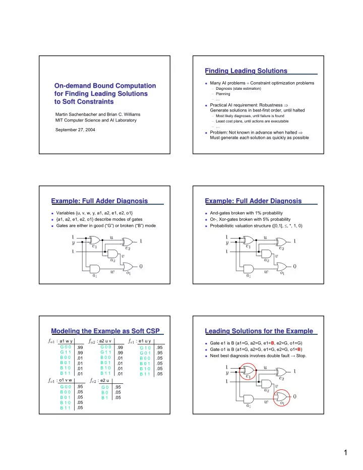
Leading Solutions for the Example Leading Solutions for the Example

Gate e1 is B (a1=G, a2=G, e1=B, e2=G, o1=G) Gate o1 is B (a1=G, a2=G, e1=G, e2=G, o1=B) Next best diagnosis involves double fault → Stop.

2

Heuristic (Bound Heuristic (Bound-

• Guided) Search

Guided) Search

Best-first (A*) search expands node with best ,

where is value so far and is heuristic estimate

(Kask Dechter AIJ 01): Compute heuristics using

bucket trees and dynamic programming A* Search Tree

Bucket Tree Bucket Tree

Scheme for one-by-one variable elimination Each node defines sub-problem with constraints

Bucket Tree Bucket Tree

Evaluate using dynamic programming Store constraint at edge to parent

Dynamic Programming Dynamic Programming Dynamic Programming Dynamic Programming Dynamic Programming Dynamic Programming

3

Bounds from Bucket Trees Bounds from Bucket Trees

Assign in reverse order using the evaluation function:

Exact Bound

Bounds from Bucket Trees Bounds from Bucket Trees Tree Decomposition Tree Decomposition

Generalization of Bucket Trees Eliminate variables in groups (partial order)

Compatible Variable Order Compatible Variable Order

Complete partial order to total order by also ordering

variables within groups (Jégou Terrioux AIJ 03)

Bounds from Tree Decompositions Bounds from Tree Decompositions

Assign in reverse order using the evaluation function:

is the node index such that Exact Bound

Bounds from Tree Decompositions Bounds from Tree Decompositions

4

On On-

• Demand Bound Computation

Demand Bound Computation

If only a few leading solutions are needed, pre-

computing becomes inefficient

Interleave search and dynamic programming to

compute only as needed (“on-demand”) Dynamic Programming Best-First Search + = On-demand Bounds

Preferential Independence Preferential Independence

For any valuation structure: Sufficient to expand only next best child Sufficient to compute only for next best child

To exploit, need to know order of children in advance

Dual Formulation Dual Formulation

Unary soft constraints (functions as variables) Binary hard constraints (equality) Compatible order

Dual Formulation Dual Formulation

Drop redundant (inter-cluster) equality constraints Preserve locality (tree structure)

Approximating H Approximating H

Drop hard (equality) constraints for H Heuristics becomes equal for all children Order of children known if tuples of fi are sorted Makes it possible to generate only as needed

On On-

• Demand Bound Computation

Demand Bound Computation

Generate tuples of constraints only as needed

Generate Next Best Tuple (Root) Generate Next Best Tuple (Child)

5

Example Example Example Example Example Example Example Example Example Example Example Example

6

Example Example Example Example Example Example Example Example Example Example Example Example

7

Example Example Example Example

Best Solution found

Experiments Experiments

Random Max-CSPs, first (best) solution

Related Approach Related Approach

BTDval algorithm (Terrioux Jégou CP 03) Depth-first branch-and-bound on tree decompositions Record tuples for constraints (“structural goods”)

Comparison Comparison

BTDval BFOB Space Time O(exp(s)) O(exp(w)) Problem Single optimal Solution Solutions in Best-first order O(exp(w)) O(exp(w)) s = Separator size, w = Tree width (s ≤ w)

Future Work Future Work

Evaluate against depth-first branch-and-bound

– Best-first (A*) search potentially faster

Combine with approximate dynamic programming

– Mini-buckets (Dechter Rish UAI 97)

Extend to partial orders

– Semiring-based CSPs (Bistarelli IJCAI 95)

8

Material Finding Finding Leading Solutions Leading Solutions

% Solutions Time Best … 2nd best Best 2nd best … 3rd best