1 Multiple problems Applying Marching Cubes (thresholding) - - PDF document

SLIDE 1

1

Level Sets

Roger Crawfis

Slides collected from: Fan Ding, Charles Dyer, Donald Tanguay and Roger Crawfis

4/24/2003

• R. Crawfis, Ohio State Univ.

109

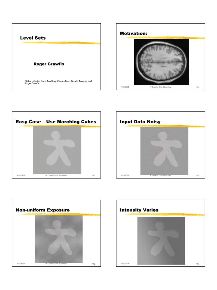
Motivation:

4/24/2003

• R. Crawfis, Ohio State Univ.

110

Easy Case – Use Marching Cubes

4/24/2003

• R. Crawfis, Ohio State Univ.

111

Input Data Noisy

4/24/2003

• R. Crawfis, Ohio State Univ.

112

Non-uniform Exposure

4/24/2003

• R. Crawfis, Ohio State Univ.

113

Intensity Varies

SLIDE 2

2

4/24/2003

• R. Crawfis, Ohio State Univ.

114

Multiple problems

4/24/2003

• R. Crawfis, Ohio State Univ.

115

Applying Marching Cubes (thresholding)

4/24/2003

• R. Crawfis, Ohio State Univ.

116

Applying A Threshold

4/24/2003

• R. Crawfis, Ohio State Univ.

117

Applying A Threshold

4/24/2003

• R. Crawfis, Ohio State Univ.

118

Four (contour) Levels

4/24/2003

• R. Crawfis, Ohio State Univ.

119

What To Do?

User Intervention!!!

We see it!! It’s right there!!! Well, the edges get pretty fuzzy .

Two step process:

• 1. Draw an initial curve (or surface) within the

desired region.

• 2. Expand that interface outward towards the

edge of our desired region.

SLIDE 3

3

4/24/2003

• R. Crawfis, Ohio State Univ.

120

Interfaces

An interface (or front) is a boundary between two regions: “inside” and “outside.” In 2-D, an interface is a simple closed curve:

4/24/2003

• R. Crawfis, Ohio State Univ.

121

Propagating Interfaces

How does an interface evolve over time? At a specific moment, the speed function F (L, G, I) describes the motion of the interface in the normal direction.

4/24/2003

• R. Crawfis, Ohio State Univ.

122

Propagating Interfaces

• Local – depend on local geometric information

(e.g., curvature and normal direction)

• Global – depend on the shape and position of the front

(e.g., integrals along the front, heat diffusion)

• Independent – do not depend on the shape of the front

(e.g., an underlying fluid velocity that passively transports the front) Speed F(L,G,I) is a function of 3 types of properties:

4/24/2003

• R. Crawfis, Ohio State Univ.

123

Motion Under Curvature

Example: Motion by curvature. Each piece moves perpendicular to the curve with speed proportional to the local curvature.

large positive motion small negative motion

4/24/2003

• R. Crawfis, Ohio State Univ.

124

Motion Under Curvature

Curvature κ is the inverse of the radius r of the osculating circle.

4/24/2003

• R. Crawfis, Ohio State Univ.

125

Motion Under Curvature

http://math.berkeley.edu/~sethian/Applets/java_curve_flow.html

SLIDE 4

4

4/24/2003

• R. Crawfis, Ohio State Univ.

126

Functional Representation

Eulerian framework: define fixed coordinate system on the world. For every world point x, there is (at most) one value y = ft(x). Falling snow example:

) (

0 x

f y

t=

= ) (

1 x

f y

t=

=

4/24/2003

• R. Crawfis, Ohio State Univ.

127

Functional Representation

However, many simple shapes are multivalued; they are not functions regardless of the orientation of the coordinate system.

4/24/2003

• R. Crawfis, Ohio State Univ.

128

Parametric Representation

Spatially parameterize the curve x by s so that at time t the curve is xt(s), where 0 ≤ s ≤ S and the curve is closed: xt(0) = xt(S). Points on initial curve. Gradient (wrt time) is the speed in normal direction. Normal is perpendicular to curve, as is curvature.

4/24/2003

• R. Crawfis, Ohio State Univ.

129

Parametric Representation

For motion under curvature, speed F depends only on local curvature κ – the equation of motion is thus: where curvature is and the normal is

2 / 3 2 2

) ( ) (

s s s ss s ss t

y x y x x y s + − = κ

[ ] [ ]

2 / 1 2 2 2 / 1 2 2

) ( ) ( ) (

s s T s s s s T s s t

y x x y y x y x x x s n + − =         + =         ∇ ∇ =

⊥ ⊥

• ),

( )) ( ( ) ( s n s F s x t

t t t

• ⋅

= ∂ ∂ κ

4/24/2003

• R. Crawfis, Ohio State Univ.

130

Particle Methods

In order to compute, discretize the parameterization into moving particles which reconstruct the front. Known under a variety of names: marker particle techniques, string methods, nodal methods. = # mesh particles

s ∆ t ∆

s S ∆ = time step = parameterization step ) , (

n i n i y

x = location of point i∆s at time n∆t ∆s

4/24/2003

• R. Crawfis, Ohio State Univ.

131

Problem Statement

Generally, given:

An initial front Equations that govern its evolution

How do we simulate the front’s evolution? Called an ‘initial value problem’

Given the initial position Solve for a position at a future time

SLIDE 5

5

4/24/2003

• R. Crawfis, Ohio State Univ.

132

More formally:

Given some initial front Г:

4/24/2003

• R. Crawfis, Ohio State Univ.

133

More formally: (2)

And a function F that specifies the velocity

• f the front in the normal direction:

4/24/2003

• R. Crawfis, Ohio State Univ.

134

More formally: (3)

Solve for Г at some future time Level set methods are used to track an interface Water/air interface, for example

4/24/2003

• R. Crawfis, Ohio State Univ.

135

What’s Wrong with the Obvious Solution?

Why is a level set method necessary? There seems to be a more intuitive way to solve this problem

4/24/2003

• R. Crawfis, Ohio State Univ.

136

Marker/String Methods

Why not just connect some control points (in 3D, triangulate):

4/24/2003

• R. Crawfis, Ohio State Univ.

137

Marker/String Methods (2)

And run the simulation on the points?

SLIDE 6

6

4/24/2003

• R. Crawfis, Ohio State Univ.

138

Ocean Waves

Think of an air/water interface with two waves racing towards each other:

4/24/2003

• R. Crawfis, Ohio State Univ.

139

Ocean Waves (2)

What happens to the control points when the waves collide?

4/24/2003

• R. Crawfis, Ohio State Univ.

140

Shocks

Event known as a ‘shock’ Below formation called a ‘swallowtail’

4/24/2003

• R. Crawfis, Ohio State Univ.

141

Shocks (2)

How to fix up the control points? Fixing swallowtails known as ‘de-looping’

Very difficult Some methods exist in 2D No robust 3D methods so far

4/24/2003

• R. Crawfis, Ohio State Univ.

142

Changing Topology

Example: two fires merge into a single fire.

4/24/2003

• R. Crawfis, Ohio State Univ.

143

Changing Topology

Buoys! In particle methods:

• Difficult (and expensive) to detect and change the particle chains
• Much more difficult as dimensionality increases

SLIDE 7

7

4/24/2003

• R. Crawfis, Ohio State Univ.

144

Difficulties With Particle Methods

Instability Local singularities Management of particles: remove, redistribute, connect

4/24/2003

• R. Crawfis, Ohio State Univ.

145

Level Set Formulation

Recast problem with one additional dimension – the distance from the interface. And then use Marching Cubes to extract the surface. ) , ( y x z

t=

= φ

4/24/2003

• R. Crawfis, Ohio State Univ.

146

Level Set Methods

Contour evolution method due to J. Sethian and

• S. Osher, 1988

www.math.berkeley.edu/~sethian/level_set.html Difficulties with snake-type methods

Hard to keep track of contour if it self-intersects during its evolution Hard to deal with changes in topology

4/24/2003

• R. Crawfis, Ohio State Univ.

147

The level set approach:

Define problem in 1 higher dimension Define level set function z = φ(x,y,t=0) where the (x,y) plane contains the contour, and z = signed Euclidean distance transform value (negative means inside closed contour, positive means outside contour)

4/24/2003

• R. Crawfis, Ohio State Univ.

148

How to Move the Contour?

Move the level set function, φ(x,y,t), so that it rises, falls, expands, etc. Contour = cross section at z = 0

4/24/2003

• R. Crawfis, Ohio State Univ.

149

Level Set Surface

The zero level set (in blue) at one point in time is a slice of the level set surface (in red)

SLIDE 8

8

4/24/2003

• R. Crawfis, Ohio State Univ.

150

Level Set Surface

Later in time the level set surface (red) has moved and the new zero level set (blue) defines the new contour

4/24/2003

• R. Crawfis, Ohio State Univ.

151

Level Set Surface

4/24/2003

• R. Crawfis, Ohio State Univ.

152

Level Set Formulation

The interface always lies at the zeroth level set of the function Φ, i.e., the interface is defined by the implicit equation Φt (x, y) = 0.

4/24/2003

• R. Crawfis, Ohio State Univ.

153

How to Move the Level Set Surface?

• 1. Define a velocity field, F, that specifies how contour

points move in time

Based on application-specific physics such as time, position, normal, curvature, image gradient magnitude

• 2. Build an initial value for the level set function,

φ(x,y,t=0), based on the initial contour position

• 3. Adjust φ over time; current contour defined by φ(x(t),

y(t), t) = 0 y Φ x Φ F t Φ Φ F t Φ

2 1 2 2

=                 ∂ ∂ +       ∂ ∂ + ∂ ∂ = ∇ ⋅ + ∂ ∂

• 4/24/2003
• R. Crawfis, Ohio State Univ.

154

Speed Function

( )

εK 1 (k) F F F(K)

1

− = + =

( ) ( )

εK 1 x,y k F(K)

I

− ∗ =

( )

( )

x,y I G

• I

σ I

σ

e k x,y I G 1 1 k

∗ ∇

= ∗ ∇ + =

4/24/2003

• R. Crawfis, Ohio State Univ.

155

Example: Shape Simplification

F = 1 – 0.1κ where κ is the curvature at each contour point

SLIDE 9

9

4/24/2003

• R. Crawfis, Ohio State Univ.

156

Example: Segmentation

Digital Subtraction Angiogram F based on image gradient and contour curvature

4/24/2003

• R. Crawfis, Ohio State Univ.

157

Example (cont.)

Initial contour specified manually

4/24/2003

• R. Crawfis, Ohio State Univ.

158

Result – segmentation using Fast marching

No level set tuning

4/24/2003

• R. Crawfis, Ohio State Univ.

159

Results – vein segmentation

No level set tuning With level set tuning

4/24/2003

• R. Crawfis, Ohio State Univ.

160

Results – vein segmentation continued

Original Our result Sethian’s result (Fast marching + (Level set only) Level set tuning) 4/24/2003

• R. Crawfis, Ohio State Univ.

161

Result – segmentation using Fast marching

No level set tuning

SLIDE 10

10

4/24/2003

• R. Crawfis, Ohio State Univ.

162

Results – brain segmentation continued

No level set tuning With level set tuning

4/24/2003

• R. Crawfis, Ohio State Univ.

163

Results – brain image segmentation

# of iterations = 9000 # of iterations = 12000 Fast marching only, no level set tuning