1 Transition Systems Basic safety problems We can recursively - - PDF document

SLIDE 1

1

Transition systems, temporal logic, refinement notions

George J. Pappas Departments of ESE and CIS University of Pennsylvania pappasg@ee.upenn.edu

http://www.seas.upenn.edu/~pappasg

DISC Summer School on Modeling and Control of Hybrid Systems Veldhoven, The Netherlands June 23-26, 2003

http://lcewww.et.tudelft.nl/~disc˙hs/

Outline of this mini-course

Lecture 1 : Monday, June 23

Examples of hybrid systems, modeling formalisms

Lecture 2 : Monday, June 23

Transitions systems, temporal logic, refinement notions

Lecture 3 : Tuesday, June 24

Discrete abstractions of hybrid systems for verification

Lecture 4 : Tuesday, June 24

Discrete abstractions of continuous systems for control

Lecture 5 : Thursday, June 26

Bisimilar control systems

Transition Systems

A transition system consists of

A set of states Q A set of events A set of observations O The transition relation The observation map

Initial or final states may be incorporated The sets Q, , and O may be infinite Language of T is all sequences of observations

) O, , Σ, Q, ( T ⋅ → =

• 2

σ 1

q q →

Σ

Σ

q

1

q

2

q

3

q

4

q

• 1
• 2
• 1
• q

=

σ σ σ σ

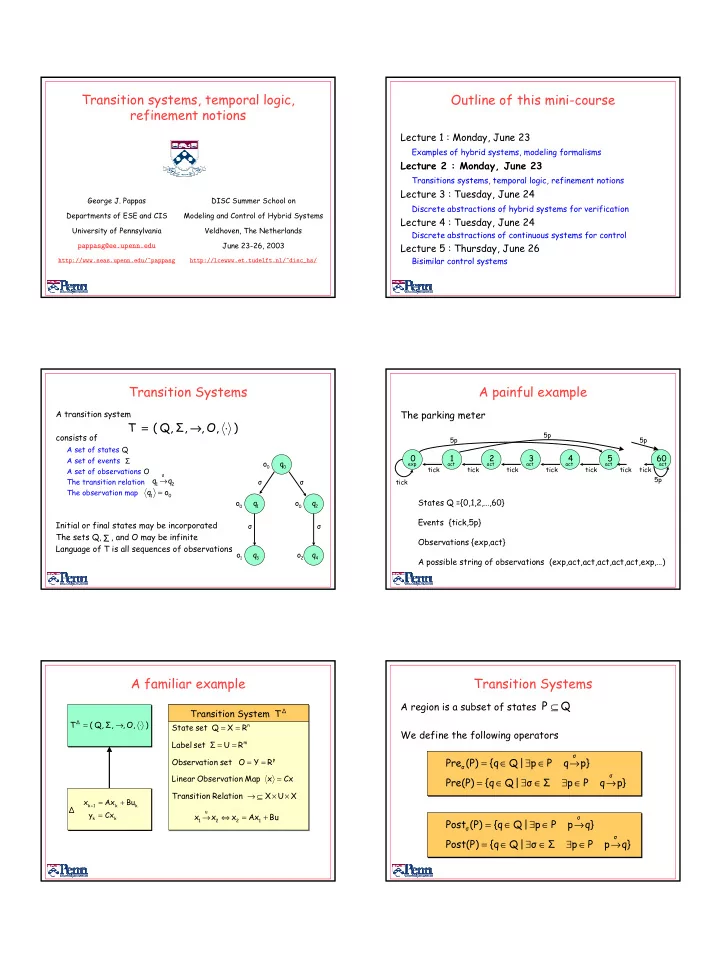
A painful example

The parking meter

1 2 3 60 4 5

tick tick tick tick tick tick tick tick 5p 5p 5p 5p

States Q ={0,1,2,…,60} Events {tick,5p} Observations {exp,act} A possible string of observations (exp,act,act,act,act,act,exp,…)

exp act act act act act act

A familiar example

1

T

∆

k k 1 k

Bu Ax x + =

+ k k

Cx y = ) O, , Σ, Q, ( T∆ ⋅ → =

n

R X Q set State = =

m

R U Σ set Label = =

p

R Y O set n Observatio = = Cx x Map n Observatio Linear = X U X Relation Transition × × ⊆ → Bu Ax x x x

1 2 2 u 1

+ = ⇔ →

∆

T System Transition

Transition Systems

A region is a subset of states We define the following operators

Q P ⊆

p} q P p | Q {q (P) Pre

σ σ

→ ∈ ∃ ∈ = p} q P p Σ σ | Q {q Pre(P)

σ

→ ∈ ∃ ∈ ∃ ∈ = q} p P p | Q {q (P) Post

σ σ

→ ∈ ∃ ∈ = q} p P p Σ σ | Q {q Post(P)

σ

→ ∈ ∃ ∈ ∃ ∈ =

SLIDE 2

2

Transition Systems

We can recursively define Similarly for the other operators. Also (P)) (Pre Pre (P) Pre

1

• n

σ σ n σ

= (P) Pre (P) Pre

σ 1 σ

=

U

N n n *

(P) Pre (P) Pre

∈

=

U

N n n *

(P) Post (P) Post

∈

=

Basic safety problems

Given transition system T and regions P, S determine Forward Forward Reachability Reachability Backward Backward Reachability Reachability

Postã(P) ∩ S6=∅ P ∩ Preã(S)6=∅

If T is finite, then algorithm terminates (decidability). Complexity :

Forward reachability algorithm

Forward Forward Reachability Reachability Algorithm Algorithm

initialize while TRUE do if return UNSAFE ; end if; if return SAFE ; end if; end while R := P

R ∩ S6=∅ R := R ∪ Post(R)

Post(R) ò R

O(nI + mR)

reachable transitions initial states

If T is infinite, then there is no guarantee of termination.

Backward reachability algorithm

Backward Backward Reachability Reachability Algorithm Algorithm

initialize while TRUE do if return UNSAFE ; end if; if return SAFE ; end if; end while R := S

R ∩ P6=∅ R := R ∪ Pre(R)

Pre(R) ò R Representation issues

Enumeration for finite sets Symbolic representation for infinite (or finite) sets

Operations on sets

Boolean operations Pre and Post computations (closure?)

Algorithmic termination (decidability)

Guaranteed for finite transition systems No guarantee for infinite transition systems

Algorithmic issues

More sophisticated properties can be expressed using

Linear Temporal Logic (LTL) Computation Tree Logic (CTL) CTL* mu-calculus

More complicated problems

SLIDE 3

3

The basic verification problem

Basic verification problem Basic verification problem

T |=ϕ

Given transition system T, and temporal logic formula ϕ Two main approaches Model checking : Algorithmic, restrictive Deductive methods : Semi-automated, general

Another verification problem

Another verification problem Another verification problem

L(T) ò L(S)

Given transition system T, and specification system S Language inclusion problems

The basic synthesis problem

Basic synthesis problem Basic synthesis problem

T k C |=ϕ

Given transition system T, and temporal logic formula ϕ Synthesis in computer science assumes disturbances Deep relationship between synthesis and game theory

Express temporal specifications along sequences Informally Syntax Semantics Eventually p Always p If p then next q p until q

Linear temporal logic (informally)

♦p p ⇒ í q p U q

qqqqqqqqqqqqp

qqqqqqqqpq pppppppppppppppq

p

pppppppppppppp

Linear temporal logic syntax The LTL formulas are defined inductively as follows Atomic propositions All observation symbols p are formulas Boolean operators If and are formulas then Temporal operators If and are formulas then

Linear temporal logic (formally)

ϕ1 ϕ2 ϕ1 ϕ2 ϕ1 ∨ ϕ2 ¬ϕ1 ϕ1 U ϕ2 í ϕ1

The LTL formulas are interpreted over infinite (omega) words

w = p0 p1 p2 p3 p4. . .

(w, i) |=p iff pi = p (w, i) |=ϕ1 ∨ ϕ2 iff (w, i) |=ϕ1 (w, i) |=ϕ1 U ϕ2 (w, i) |= í ϕ1 iff (w, i + 1)|=ϕ1

• r (w, i) |=ϕ2

(w, i) |=¬ϕ1 iff (w, i) 6 |=ϕ1

Linear temporal logic semantics

∃j õ i (w, j) |=ϕ2 and ∀ i ô k ô j (w, k) |=ϕ2 w |=þ iff (w, 0) |= ϕ T |=þ iff ∀w ∈ L(T) w |= ϕ

SLIDE 4

4

Syntactic boolean abbreviations Conjunction Implication Equivalence Syntactic temporal abbreviations Eventually Always In 3 steps

Linear temporal logic

♦ ϕ = > U ϕ ϕ = ¬♦ ¬ϕ ϕ1 ∧ ϕ2 = ¬(¬ϕ1 ∨ ¬ϕ2) ϕ1 ⇒ ϕ2 = ¬ϕ1 ∨ ϕ2 ϕ1 ⇔ ϕ2 = (ϕ1 ⇒ ϕ2) ∧ (ϕ2 ⇒ ϕ1) í3 ϕ = í í í ϕ

Two processors want to access a critical section. Each processor can has three

• bservable states

p1={inCS, outCS, reqCS} p2={inCS, outCS, reqCS} Mutual exclusion Both processors are not in the critical section at the same time. Starvation freedom If process 1 requests entry, then it eventually enters the critical section.

LTL examples

¬(p1 = inCS ∧ p2 = inCS) p1 = reqCS ⇒ ♦p1 = inCS

LTL Model Checking

LTL model checking LTL model checking

T |=ϕ

Given transition system and LTL formula we have LTL model checking is decidable for finite T Complexity : Determine if

O((n + m)(k + l)2O(k))

states transitions formula length

System verified Counterexample

Express specifications in computation trees (branching time) Informally Syntax Semantics Inevitably next p Possibly always p

Computation tree logic (informally)

∀ í p ∃ p p p p p q p q

Comparing logics

LTL CTL CTL*

Dealing with complexity

Bisimulation Simulation Language Inclusion

SLIDE 5

5

Language Equivalence

Consider two transition systems and over same and O Languanges are equivalent L( )=L( )

• p

3

p

4

p

• 1
• 2
• 1

T

2

T Σ

2

T

• q

1

q

2

q

3

q

4

q

• 1
• 2
• 1

T

σ σ σ σ σ σ σ

1

p

1

T

2

T

LTL equivalence

Consider two transition systems and and an LTL formula

Language equivalence and inclusion are difficult to check

1

T

2

T Language equivalence Language equivalence

If L(T1) = L(T2) then T1 |=ϕ ⇔ T2 |=ϕ

Language inclusion Language inclusion

If L(T1) ò L(T2) then T2 |=ϕ ⇒ T1 |=ϕ Simulation Relations

Consider two transition systems

• ver the same set of labels and observations. A relation

is called a simulation relation if it

• 1. Respects observations
• 2. Respects transitions

If a simulation relation exists, then

) O, , Σ, , Q ( T

1 1 1 1

⋅ → = ) O, , Σ, , Q ( T

2 2 2 2

⋅ → =

2 1

Q Q S × ⊆

2 1

p q then S p) (q, if = ∈ S ) p' , (q' some for p' p then , q' q and S p) (q, if

σ σ

∈ → → ∈

2 1

T T ≤

Game theoretic semantics

Simulation is a matching game between the systems Check that but it is not true that

• p

3

p

4

p

• 1
• 2
• 2

T

• q

1

q

2

q

3

q

4

q

• 1
• 2
• 1

T

σ σ σ σ σ σ σ

1

p

2 1

T T ≤

1 2

T T ≤

The parking example

The parking meter A coarser model

1 2 3 60 4 5

tick tick tick tick tick tick tick tick 5p 5p 5p 5p

exp act act act act act act

5p tick tick

exp

many

5p

act

tick

many)} (60, many),..., (1, {(0,0), S =

Simulation relations

Consider two transition systems and

Complexity of Complexity of

1

T

2

T Simulation implies language inclusion Simulation implies language inclusion

If T1 ô T2 then L(T1) ò L(T2)

L(T1) ò L(T2) O((n1 + m1)2n2) T1 ô T2 O((n1 + m1)(n2 + m2))

SLIDE 6

6

Two important cases

Abstraction Refinement

2 1

T T ≤

1

T

2

T

2 1

T T ≤

1

T 2

T Bisimulation

Consider two transition systems and

Bisimulation is a symmetric simulation Strong notion of equivalence for transition systems

1

T

2

T Bisimulation Bisimulation

T1 ñ T2 if T1 ô T2 ∧ T2 ô T1

CTL* (and LTL) equivalence CTL* (and LTL) equivalence

If T1 ñ T2 then T1 |=ϕ ⇔ T2 |=ϕ If T1 ñ T2 then L(T1) = L(T2)

≈ ≤ / T T

T

≈ / T

Special quotients

Abstraction When is the quotient language equivalent or bisimilar to T ?

Quotient Transition Systems

Given a transition system and an observation preserving partition , define naturally using

• 1. Observation Map
• 2. Transition Relation

) O, , Σ, Q, ( T ⋅ → =

Q Q × ⊆ ≈

) O, , Σ, , Q/ ( T/

≈ ≈

⋅ → ≈ = ≈

• p

with P p exists there iff

• P

= ∈ =

≈

p' p with P' p' P, p exists there iff P' P

σ σ

→ ∈ ∈ → ≈

Bisimulation Algorithm

Quotient system always simulates the original system When does original system simulate the quotient system ?

≈ / T T

T ≈ / T

1

• 2
• σ

σ

Bisimulation Algorithm

Quotient system always simulates the original system When does original system simulate the quotient system ?

≈ / T T

T ≈ / T

1

• 2
• σ

σ

SLIDE 7

7

If T is finite, then algorithm computes coarsest quotient. If T is infinite, there is no guarantee of termination

Bisimulation algorithm

Bisimulation Bisimulation Algorithm Algorithm

initialize while such that end while Q/ø = {p ø q iff < q >=< p >}

∅6= ò P ∩ Pre(P0)6= ò P0

P1 := P ∩ Pre(P0)

∃P, P0 ∈ Q/ø

P2 := P \ Pre(P0) Q/ø := (Q/ø \ {P}) ∪ {P1, P2}

Relationships

Bisimulation Simulation Language Inclusion

Strongest, more properties, easiest to check Weaker, less properties, easy to check Weakest, less properties, difficult to check

Complexity comparisons

Bisimulation Simulation Language Equivalence

O(m á log(n)) O(m á n) O(m á 2n)

≈ ≡ / T T

T

≈ / T

Discrete to discrete

Abstraction Goal : Complexity reduction, theoretical guarantees Discrete Discrete

≈ ≡ / T T

T

≈ / T

Continuous to discrete (Lectures 3 & 4)

Abstraction Goal : Algorithmic feasibility, decidability, property dependent quantization Continuous Hybrid Discrete

≈ ≡ / T T

T

≈ / T

Continuous to continuous (Lecture 5)

Abstraction Goal : Property dependent reduction, hierarchical control, search for a unified systems theory Continuous Continuous