1
play

1 Ray Tracing Avoiding Ray Traced Look Ray Tracing - Problems - PDF document

Paper Summaries Any takers? Advanced Ray Tracing Assignments Projects Project feedback Checkpoint 5 Approx 18 projects Due next monday Listing of projects now on Web Checkpoint 6 Presentation schedule


  1. Paper Summaries • Any takers? Advanced Ray Tracing Assignments Projects • Project feedback • Checkpoint 5 • Approx 18 projects – Due next monday • Listing of projects now on Web • Checkpoint 6 • Presentation schedule – To be given next monday – Presentations (15 min max) • RenderMan – Last 3 classes (week 10 + finals week) – Due February 16th – Sign up • Email me with 1 st , 2 nd , 3 rd choices • First come first served. Ray Tracing 
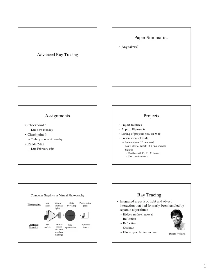
Computer Graphics as Virtual Photography • Integrated aspects of light and object real camera photo Photographic Photography: interaction that had formerly been handled by scene (captures processing print light) separate algorithms: – Hidden surface removal processing – Reflection – Refraction camera Computer 3D synthetic tone model Graphics: models reproduction image – Shadows (focuses – Global specular interaction simulated Turner Whitted lighting) 1

  2. Ray Tracing – Avoiding Ray Traced Look Ray Tracing - Problems • Object - ray intersection • Avoiding that “ray traced look” , i.e., handle • Ray traced images are point sampled diffuse interaction – “Too sharp” (super real) – “wrong image” – Ray tracing is point sampling – Sharp shadows • 1 ray per pixel – Sharp Reflection/Refraction • Multiple reflections especially are too sharp – Assumes pixel is a single point – Aliasing – Assumes pin hole camera • Doesn’t handle major light transport functions • 1 ray for transmission & reflection – Diffuse interaction – Assumes all reflection is specular – Scattering of light – Assumes that BRDF for all incoming directions is single out going direction – Caustics • Computation time Ray Tracing – Avoiding Ray Traced Look Ray Tracing – Avoiding Ray Traced Look • Three approaches – “Backward” ray tracing – Trace objects other than rays – Stochastic sampling [Watt/Watt,251] Tracing things other than rays “Backward”/ “Reverse” Ray Tracing • Beam tracing – pyramidal beams This approach is – Recursively applies Weiler-Atherton hidden (sort of) used in surface removal algorithm Photon Mapping – Polygonal surfaces only also – later… • Cone tracing – cones • Pencil Tracing – bundle of rays – Paraxial rays -> 4D vectors – Requires smooth surfaces [Watt/Watt,250] 2

  3. Tracing things other than rays Tracing things other than rays [Heckbert84] Tracing things other than rays Cone Tracing Examples • Same as traditional ray tracing except – Intersection is a surface – Surfaces spawn more cones, beams, pencils – Advantage: More realistic – Disadvantage: Increase in complexity of geometric calculations • e.g., in cone tracing, calculations not only involve an http://www.cs.uaf.edu/~ genetti/ intersection, but also the ratio between the cross-section of beam and area of intersection of object is needed Note the fuzzy reflections and soft shadows Stochastic Ray Tracing Distributed Ray Tracing • Introduced by Cook, Porter, Carpenter in 1984. • Introduce randomness in ray spawning • Unified • Kajiya86 used for solving rendering – Blurred reflections equation – Blurred refraction – Soft shadows – Either reflection or refraction is spawned – Depth of field – Reflection rays can be spawned in diffuse – Motion blur Loren Carpenter Rob Cook direction • Uses stochastic sampling to get rid of ray traced look. – Multiple “paths” per pixel • Uses ray bundle, but size limited stochastically 3

  4. Distributed Ray Tracing Distributed Ray Tracing • “Jitter” sampling – Trades aliasing for noise! – Use Poisson “noise” to jitter values from original “fixed” position – Using “jittering” in • Initial ray generation • Reflection/transmission ray generation • Shadow ray generation • Jitter over time. [Foley/Van Dam,788] Distributed Ray Tracing Distributed Ray Tracing • Initial ray generation – Supersample - instead of 1 ray per pixel, shoot Poisson Jittering 16 rays per pixel. Jittered regular – no pair closer distribution – Initial ray positions are not evenly spaced, than a min. distance rather distributed stochastically within pixel using “jittering” [Foley/Van Dam,789] Distributed Ray Distributed Ray Tracing Tracing Depth of Field • Jittered ray generation – Using a lens/camera model Notice different – Simulation of depth of field size circles of confusion caused – First use of non-pinhole camera model in ray by different sized tracing lens [Watt/Watt,264] 4

  5. Distributed Ray Tracing Distributed Ray Tracing Depth of Field • Jittered ray generation [Watt/Watt,264] [Cook84] Distributed Ray Tracing Distributed Ray Tracing • Jittered Reflection • Jittered Reflection – Send out multiple rays jittered about the real reflection direction – Contribution of each ray to intensity weighted by a predefined “importance” function - associated with the object’s reflectance properties [Watt/Watt,263] Jittered Reflection Jittered Transmission 1 reflection ray 10 reflection rays 20 reflection rays 50 reflection rays 1 transmission ray 10 transmission rays 20 transmission rays Allen Martin, WPI Allen Martin, WPI 5

  6. Distributed Ray Tracing Distributed Ray Tracing Soft Shadows • Jittered shadow rays – Multiple jittered rays sent out toward light sources – Contribution of each determined by a predefined importance function - associated with the light – Shadow rays return fraction of light seen rather than yes/no – Results in soft shadows [Cook84] Jittered Shadow Rays Distributed Ray Tracing • Jittering in time – Do ray tracing over a duration of time in which objects may move. – Uses same rays repeatedly over time interval 1 shadow ray 10 shadow rays 20 shadow rays – Results in motion blur Allen Martin, WPI Distributed Ray Tracing Distributed Ray Tracing - Summary Motion Blur • Stochastic sampling (“jitter sampling”) • Apply jittering to: – Initial ray selection • Jittering on image plane + use of camera/lens model – Reflection / Transmittance – Shadow Rays – Over time [Cook84] 6

  7. Photon Mapping Photon Mapping - Motivation • Combines “backward”/ “reverse” ray tracing with stochastic ray tracing • Used to simulate the interaction of light with a variety transparent substances (caustics) – Glass – Water – Diffuse Inter-reflections between illuminated objects – Effects of particulate matter • Smoke • Water vapor Without With Photon Mapping Photon Mapping - Caustics • Pattern of light focused on a surface after having • Henrik Wann Jensen 95/96 original light path bent by intermediate surface. • Simulates the transport of • For example, a glass of wine on a table changes the individual photons emitted pattern and the color of light from light sources • Photons bounce off specular surfaces • Photons deposited on diffuse surfaces • Photons collected by ray tracing from eye [Jensen] Photon Mapping Algorithm • Photon tracing Photon Mapping – Light packets sent from light sources – When intersect surface, store in photon map : • 3D coordinate of intersection • Incoming direction • Energy – Energy absorbed on bounces and refraction – Monte Carlo – Similar to reverse ray tracing • Rendering – Ray tracing for direct illumination – Object intersected by ray • Check if in range of stored photons – yes, add energy – Photon map visualization • Indirect bounce [Slide by John Hart] 7

  8. Photon Map The Light of Mies van der Rohe • A photon map is a data structure that stores all distributed photons • Often three photon maps are used – One for caustics – One for indirect illumination – One for volume caustics • For efficiency, photon direction is often constrained – Only sent in direction of objects known to cause caustics 2000ET Photon Mapping the Cornell Box Photon Mapping - Summary • Combines “backward”/ “reverse” ray tracing with stochastic ray tracing to generate caustics • Cost effective compared to other methods Using Photon Mapping. Resolution Using Radiance. Resolution 5120x3840. Ray traced Photon mapped 2560x1920. Rendering time 50 Rendering time 6 hours. min. Parallel Computing Parallel Hardware • What is it? • SIMD – Solving a problem by dividing it into tasks to – Same instruction executed in be handled by separate processors lockstep fashion on different data • Why use it? • MIMD – Performance – Different instructions executed – Goal linear speedup on different data • MIMD-SM • MIMD-DM 8

Download Presentation
Download Policy: The content available on the website is offered to you 'AS IS' for your personal information and use only. It cannot be commercialized, licensed, or distributed on other websites without prior consent from the author. To download a presentation, simply click this link. If you encounter any difficulties during the download process, it's possible that the publisher has removed the file from their server.

Recommend


More recommend