1 matrix notation and preliminaries from spectral graph
play

1 Matrix notation and preliminaries from spectral graph theory - PDF document

CS 224W Graph clustering Austin Benson Graph clustering (or community detection or graph partitioning) is one of the most studied problems in network analysis. One reason for this is that there are a variety of ways to define a cluster


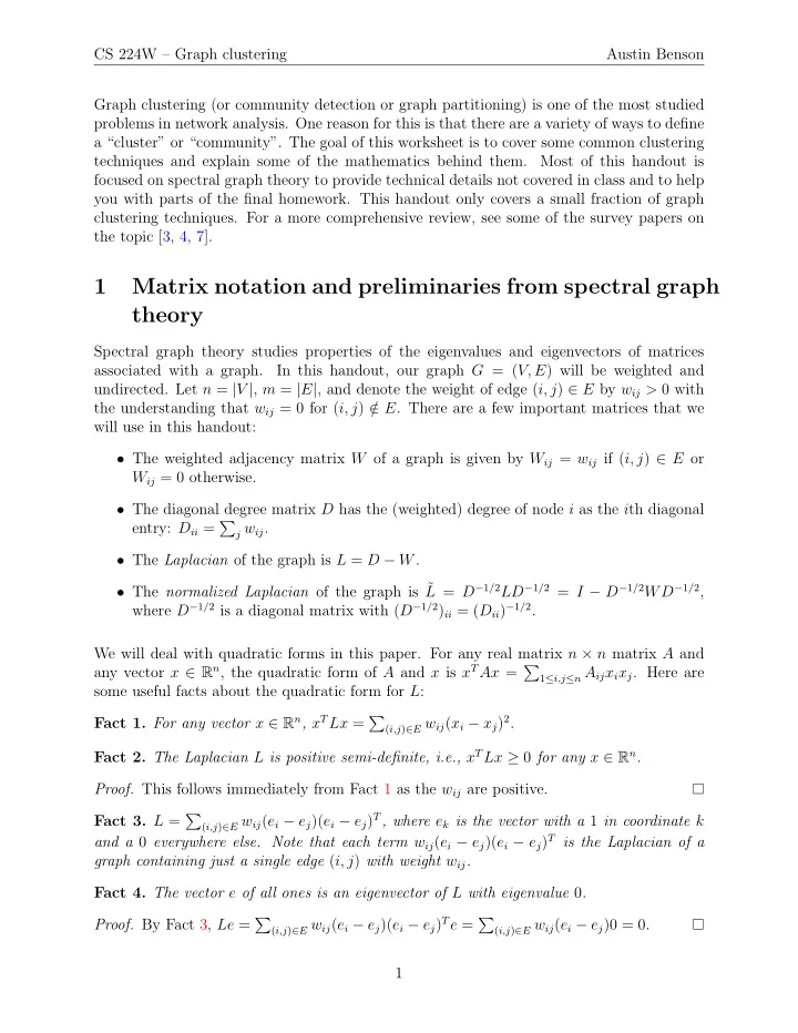
  1. CS 224W – Graph clustering Austin Benson Graph clustering (or community detection or graph partitioning) is one of the most studied problems in network analysis. One reason for this is that there are a variety of ways to define a “cluster” or “community”. The goal of this worksheet is to cover some common clustering techniques and explain some of the mathematics behind them. Most of this handout is focused on spectral graph theory to provide technical details not covered in class and to help you with parts of the final homework. This handout only covers a small fraction of graph clustering techniques. For a more comprehensive review, see some of the survey papers on the topic [3, 4, 7]. 1 Matrix notation and preliminaries from spectral graph theory Spectral graph theory studies properties of the eigenvalues and eigenvectors of matrices associated with a graph. In this handout, our graph G = ( V, E ) will be weighted and undirected. Let n = | V | , m = | E | , and denote the weight of edge ( i, j ) ∈ E by w ij > 0 with the understanding that w ij = 0 for ( i, j ) / ∈ E . There are a few important matrices that we will use in this handout: • The weighted adjacency matrix W of a graph is given by W ij = w ij if ( i, j ) ∈ E or W ij = 0 otherwise. • The diagonal degree matrix D has the (weighted) degree of node i as the i th diagonal entry: D ii = � j w ij . • The Laplacian of the graph is L = D − W . L = D − 1 / 2 LD − 1 / 2 = I − D − 1 / 2 WD − 1 / 2 , • The normalized Laplacian of the graph is ˜ where D − 1 / 2 is a diagonal matrix with ( D − 1 / 2 ) ii = ( D ii ) − 1 / 2 . We will deal with quadratic forms in this paper. For any real matrix n × n matrix A and any vector x ∈ R n , the quadratic form of A and x is x T Ax = � 1 ≤ i,j ≤ n A ij x i x j . Here are some useful facts about the quadratic form for L : Fact 1. For any vector x ∈ R n , x T Lx = � ( i,j ) ∈ E w ij ( x i − x j ) 2 . Fact 2. The Laplacian L is positive semi-definite, i.e., x T Lx ≥ 0 for any x ∈ R n . Proof. This follows immediately from Fact 1 as the w ij are positive. ( i,j ) ∈ E w ij ( e i − e j )( e i − e j ) T , where e k is the vector with a 1 in coordinate k Fact 3. L = � and a 0 everywhere else. Note that each term w ij ( e i − e j )( e i − e j ) T is the Laplacian of a graph containing just a single edge ( i, j ) with weight w ij . Fact 4. The vector e of all ones is an eigenvector of L with eigenvalue 0 . ( i,j ) ∈ E w ij ( e i − e j )( e i − e j ) T e = � Proof. By Fact 3, Le = � ( i,j ) ∈ E w ij ( e i − e j )0 = 0. 1

  2. CS 224W – Graph clustering Austin Benson By Fact 2, all of the eigenvalues of L are nonnegative, so Fact 4 says that an eigenvector corresponding to the smallest eigenvalue of L is the vector of all ones (with eigenvalue 0). Since L is symmetric, it has a complete eigendecomposition. In general, we will denote the eigenvalues of L by 0 = λ 1 ≤ λ 2 ≤ . . . λ n − 1 ≤ λ n . It turns out that the zero eigenvalues determine the connected components of the graph: Fact 5. If G has exactly k connected components, then 0 = λ 1 = λ 2 . . . = λ k < λ k +1 In other words, the first k eigenvalues are 0 , and the ( k + 1) st eigenvalue is positive. 2 Fiedler vector The Fiedler vector is the eigenvector corresponding to the second smallest eigenvalue of the graph Laplacian and dates back to Fiedler’s work on spectral graph theory in the 1970s [2]. In other words, the Fiedler vector v satisfies Lv = λ 2 v (side note: λ 2 is called the algebraic connectivity of the graph G ). The Fiedler vector may be used for partitioning a graph into two components. Here we present the derivation of Riolo and Newman [6]. Suppose we want to partition G into two well-separated components S and ¯ S = V \ S . A natural measure of the “separation” between S and ¯ S is the sum of the weight of edges that have one endpoint in S and one end point in ¯ S . This is commonly referred to as the cut : � cut( S ) = w ij (1) i ∈ S,j ∈ ¯ S Note that the cut measure is symmetric in S and ¯ S , i.e., cut( S ) = cut( ¯ S ). We can relate the cut to a quadratic form on L with an assignment vector x on the sets. Specifically, let x be an assignment vector: � 1 node i ∈ S x i = (2) node i ∈ ¯ − 1 S Then w ij ( x i − x j ) 2 = � � � x T Lx = w ij 4(1 − I x i = x j ) = 8 w ij = 8 · cut( S ) (3) i ∈ S,j ∈ ¯ ( i,j ) ∈ E ( i,j ) ∈ E S At first glance, we might just want to find an assignment vector x that minimizes the cut value. If we assign all nodes i to S then we get a cut value of 0, which is clearly the minimum. However, this is not an interesting partition of the graph. We would like to enforce some sort of balance in the partition. One approach is to minimize the cut under the constraint that S has exactly half the nodes (assuming the graph has an even number of nodes). In this case, we have that � � � ( − 1) = | S | − | ¯ x i = 1 + S | = 0 . i ∈ ¯ i i ∈ S S 2

  3. CS 224W – Graph clustering Austin Benson In matrix notation, we can write this as x T e = 0, where e is the vector of all ones. This leads to the following optimization problem x T Lx minimize x x T e = 0 subject to x i ∈ {− 1 , 1 } Unfortunately, the constraint that the x i take the value − 1 or +1 makes the optimization NP-hard [10]. Thus, we use a common trick in combinatorial optimization: (i) relax the constraints to a tractable problem and (ii) round the solution from the relaxed problem to a solution in the original problem. In this case, we will relax the constraint that x i ∈ {− 1 , 1 } to the constraint x ∈ R with x T x = n . Note that the latter constraint is always satisfied in our original optimization problem—we use it here to get a bound on the size of x in the relaxed problem. Our new relaxed optimization problem is: x T Lx minimize x x T e = 0 (4) subject to x T x = n It turns out that the Fiedler vector solves this optimization problem: Theorem 6. Let G be connected. The minimizer of the optimization problem in Equation 4 is the Fiedler vector. Proof. Since L is symmetric, there is an orthonormal basis for R n consisting of eigenvectors of L . Thus, we can write any vector x ∈ R n as n � x = w i v i , i =1 where the w i are weights and Lv i = λ i v i . Furthermore, since G is connected, there is a single basis vector that spans the eigenspace corresponding to eigenvalue 0. By Fact 4, this vector √ n e , where e is the vector of all ones. Since x T e = 0, we must have that 1 is v 1 = e/ � e � 2 = w 1 = 0 for any feasible solution, i.e., x = � n i =2 w i v i . It is easy to show that n � x T x = w 2 i i =2 and n � x T Lx = w 2 i λ i i =2 Thus, the optimization problem becomes n � w 2 minimize i λ i w 2 ,...,w n i =2 n � w 2 subject to i = n i =2 3

  4. CS 224W – Graph clustering Austin Benson Clearly, we should put all of the “mass” on λ 2 , the smallest of the eigenvalues that are non-zero. Thus, the minimizer has the weights w 2 = √ n , w 3 = w 4 = . . . w n = 0. The above theorem shows how to solve the “relaxed” problem, but we still have to round 1 the solution vector √ n v 2 to a partition of the graph. There are a couple ways we might do this. We could just assign the nodes corresponding to the positive entries of the eigenvector to S and the nodes corresponding to the negative entries to ¯ S . Alternatively, we could run k -means clustering (with k = 2) on the n real-valued points given by the eigenvector. 3 Multi-way spectral clustering with Ratio cut In general, we might want to simultaneously find k clusters of nodes instead of just finding a partition of the graph. To do this, we will try to minimize the ratio cut objective, following the derivation in [9]. Consider k disjoint sets of nodes S 1 , S 2 , . . . , S k such that ∪ k i =1 S i = V . The ratio cut is k cut( S i ) � RatioCut( S 1 , . . . , S k ) = (5) | S i | i =1 Trying to minimize the ratio cut is a sensible approach. We want each cluster S i to be well separated but not too small; thus, we minimize the ratios of cut to size for each cluster. Suppose we have an assignment matrix X such that 1 � √ node i ∈ S r | S r | X ir = (6) 0 otherwise Let x r be the r th column of X . Then � x T w ij ( x ir − x jr ) 2 r Lx r = ( i,j ) ∈ E 1 � = 2 · w ij | S r | i ∈ S r ,j ∈ ¯ S r = 2 · cut( S r ) . | S r | Recall that the trace of a matrix A , denoted tr( A ) is the sum of the diagonal entries of A . We have that k � x T r Lx r = tr( X T LX ) ∝ RatioCut( S 1 , . . . , S k ) (7) r =1 We claim that our assignment matrix X is orthogonal, i.e., that X T X = I , the identity matrix. Indeed, n n 1 � � ( X T X ) rr = x 2 ir = I i ∈ S r | S r | = 1 i =1 i =1 4

Download Presentation
Download Policy: The content available on the website is offered to you 'AS IS' for your personal information and use only. It cannot be commercialized, licensed, or distributed on other websites without prior consent from the author. To download a presentation, simply click this link. If you encounter any difficulties during the download process, it's possible that the publisher has removed the file from their server.

Recommend


More recommend