1. Here we will develop a simple Navier-Stokes solver for - - PowerPoint PPT Presentation

SLIDE 1

DNS of Multiphase Flows Gretar Tryggvason

Direct Numerical Simulations of Multiphase Flows-3
 


A Simple Solver for Variable Density Flow (1 of 3)

• 1. Here we will develop a simple Navier-Stokes solver for incompressible flows of two fluids that have

different material properties. The code is developed in several steps, adding capabilities in small increments.

DNS of Multiphase Flows A simple method to solve the Navier- Stokes equations for variable density Start by advecting density using an advection/diffusion equation This density advection will later be replaced by front tracking

• 2. The code uses explicit time integration, implemented as the so-called projection method, and a

regular structured staggered grid for a rectangular domain. We start by developing the code for flow where the viscosity is constant and there is no surface tension, and the density, which also serves as a marker to identify the different fluids, is updated by solving an advection-diffusion equation. The diffusion is added for numerical purpose and is removed once we have introduced front tracking to follow the interface between the different fluids.

DNS of Multiphase Flows

∂ ∂t Z

V

ρudv + I

S

ρuu · nds = I

S

pnds + Z

V

ρgdv + I

S

µ

• ru + (ru)T

· nds + Z

V

fdv I

S

u · nds = 0 Z Dρ Dt = ∂ρ ∂t + u · rρ = 0

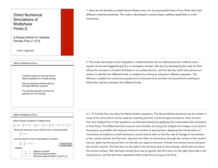
And the density of each fluid particle is constant Where the pressure is such that the flow is incompressible Navier-Stokes equations in integral form Notation

ρ u p ρh uh ph ρi,j ui,j pi,j

Original variables Numerical approximation Numerical approximation at point (i,j)

V: Control volume S: Control surface

3-1. To find the flow we solve the Navier-Stokes equations. The Navier-Stokes equations can be written in many forms, all of which can be used as a starting point for numerical approximations. Here we start from the integral form of the equations, as obtained directly by applying the conservation laws of physics to fluid flows. The differential form may be more familiar, but using the integral form keeps us as close to the physics as possible and requires minimum number of assumptions. Applying the conservation of momentum principle to a small stationary control volume tells us that the rate of change of momentum in the control volume, the first term, plus the net inflow of momentum through the surface of the control volume, given by the second term on the left, are equal to the sum of body and volume forces acting on the control volume. The first term on the right is the net force due to the pressure, which acts normal to the control surface, then we have a body force due to gravity, the third term on the right hand side is the viscous force, and the last term represents other body force acting on the fluid.

SLIDE 2

DNS of Multiphase Flows

∂ ∂t Z

V

ρudv + I

S

ρuu · nds = I

S

pnds + Z

V

ρgdv + I

S

µ

• ru + (ru)T

· nds + Z

V

fdv I

S

u · nds = 0 Z Dρ Dt = ∂ρ ∂t + u · rρ = 0

And the density of each fluid particle is constant Where the pressure is such that the flow is incompressible Navier-Stokes equations in integral form Notation

ρ u p ρh uh ph ρi,j ui,j pi,j

Original variables Numerical approximation Numerical approximation at point (i,j)

V: Control volume S: Control surface

3-2. The last term will include the surface tension, but for now we leave it unspecified. We assume that the flow is incompressible so its volume is conserved. For a control volume this means that the inflow must balance outflow, or that the integral of the normal velocity over the control surface must be zero. Incompressibility is a consequence of the density of each fluid particle remaining constant and for multiphase flows, where the density of different fluid particles is different, this means that the advection equation for the density must be included in the set of equations we need to solve. Finally, since we are sometimes dealing with the continuous flow field and sometimes with discrete approximations we need to establish a notation that distinguishes between those two. Here we use variables without a super or sub script for the continuous variables, such as rho, p and bold u, for the density, pressure and velocity, and variables with subscripts and superscripts for the discrete approximations.

DNS of Multiphase Flows

∂ ∂t Z

V

ρudv + I

S

ρuu · nds = I

S

pnds + Z

V

ρgdv + I

S

µ

• ru + (ru)T

· nds + Z

V

fdv I

S

u · nds = 0 Z Dρ Dt = ∂ρ ∂t + u · rρ = 0

And the density of each fluid particle is constant Where the pressure is such that the flow is incompressible Navier-Stokes equations in integral form Notation

ρ u p ρh uh ph ρi,j ui,j pi,j

Original variables Numerical approximation Numerical approximation at point (i,j)

V: Control volume S: Control surface

3-3. A superscript denotes a time level and a subscript denotes a discretization in space. We will use the subscript h for an unspecified spatial discretization and i,j for variables discretized on regular structured two-dimensional grids.

DNS of Multiphase Flows Similarly, the incompressibility conditions is The average value of each term, over the control volume:

∂ ∂t Z

V

ρudv + I

S

ρuu · nds = I

S

pnds + Z

V

ρgdv + I

S

µ

• ru + (ru)T

· nds + Z

V

fdv V: Control volume S: Control surface

The Navier-Stokes equations are then:

Mh = 1 V Z

V

ρudv I Z Ah = 1 V I

S

ρu(u · n)ds Z Z Dh = 1 V I

S

µru + (ru)T · n ds rhph = 1 V I

S

pn ds I fh = 1 V Z

V

fdv I rh · uh = 1 V I

S

u · nds Z Z ρhg = 1 V Z

V

ρgdv I ∂ ∂tMh = Ah rhph + ρhg + Dh + fh I

• 4. To simplify the notation we divide the integral statement of the momentum conservation by the

volume of the control volume and then define the average momentum, M, the average advection term, A, the average pressure gradient, the average gravity force---average rho times g, the average viscous term D, and the average integral of other forces f. Notice that we denoted the average pressure gradient slightly differently than the other terms to emphasize the fact that the integral is the definition

• f the pressure gradient in the limit of infinitesimal control volume. The momentum equation can now be

written in terms of these definitions, giving us the time derivative of the momentum equal to the negative of the advection terms, and the sum of the forces. Similarly, will denote the average of the conservation of volume integral as the divergence of the velocity since the divergence can be defined by this integral as the volume goes to zero.

SLIDE 3

DNS of Multiphase Flows

The Time Derivative

• 5. Because we have to solve several equations, the momentum equations along with the

incompressibility condition and the advection equation for the density, we need to decide exactly in what order to solve the equations. To do that, we start by the time integration.

DNS of Multiphase Flows Supplemented by: The semi-discrete Navier-Stokes equations then become:

e Mn

h = ρn hun h

d Mn+1

h

= ρn+1

h

un+1

h

. rh · un+1

h

= 0 uh = 1 V Z

V

udv Z ρh = 1 V Z

V

ρdv

Decompose the momentum into density and velocity and Where

This implies that the velocity and the density are slowly varying

ρn+1

h

un+1

h

ρn

hun h

∆t = An

h rhph + ρn hg + Dn h + f n h

at at

( )n : t ( )n+1 : t + ∆t

Notation

• 6. The Navier-Stokes equations give us the time evolution of the momentum, but we need the velocity

and the density separately to be able to calculate the various terms on the right hand side. Thus we assume that we can decompose the momentum into the product of the average density and the average velocity, defined by integrals over the control volume. For very small control volumes where the density and velocity are essentially constant this is obviously a very reasonable thing to do but for flows where the density changes abruptly, this is a more questionable approach, and we will revisit this approximation in later lectures. We now approximate the time derivative by a simple forward in time Euler approximation, where the right hand side is computed at the current time. Here, superscript n denotes a variable at the current time t and superscript n+1 stands for the variable at time t plus delta t. Notice that we have not put any superscript on the pressure term because the pressure needs to take whatever value required to enforce incompressibility at the new time, n+1.

DNS of Multiphase Flows To integrate in time we approximate the time derivative by a simple first order in time forward approximation: Predictor: Corrector: The pressure must ensure that Projection Method Then we split it into two steps:

rh · un+1

h

= 0 ρn+1

h

un+1

h

ρn+1

h

u∗

h

∆t = rhph ρn+1

h

un+1

h

ρn

hun h

∆t + An

h = rhph + gn h + Dn h + f n h

ρn+1u∗

h ρnun h

∆t = An

h + ρn hg + Dn h + f n h

7-1. We start by assuming that we have already updated the density so rho at time level n+1 is given. However, even if the new density is given, we cannot use the momentum equation as written to find the new velocity because we do not know the pressure. For incompressible flow this is a standard problem. We have two equations for the velocity, the momentum equation and the incompressibility condition, but no equation for the pressure. To deal with this we use the so-called projection method, where we first find a preliminary velocity field by ignoring the pressure and then determine the pressure required to make the velocity field incompressible. That is, in the second step we project the velocity onto the space of incompressible velocity fields. Thus, the name. The semi-discrete momentum equation is therefore split into two parts by adding and subtracting a term including a temporary velocity, denoted by u star. Here we assume that the temporary velocity is multiplied by the new density, but other choices are possible.

SLIDE 4

DNS of Multiphase Flows To integrate in time we approximate the time derivative by a simple first order in time forward approximation: Predictor: Corrector: The pressure must ensure that Projection Method Then we split it into two steps:

rh · un+1

h

= 0 ρn+1

h

un+1

h

ρn+1

h

u∗

h

∆t = rhph ρn+1

h

un+1

h

ρn

hun h

∆t + An

h = rhph + gn h + Dn h + f n h

ρn+1u∗

h ρnun h

∆t = An

h + ρn hg + Dn h + f n h

7-2. The first step gives us the temporary velocity using everything on the right hand side except the pressure and the second step corrects the temporary velocity by adding the pressure gradient. Adding step one and two, eliminating the temporary velocity, gives us the semi-discrete momentum equation. The pressure is still unknown, but it must be determined in such a way that the velocity at time level n+1 is incompressible, or divergence free.

DNS of Multiphase Flows By taking the divergence of and using we obtain the pressure equation We will take the last step using the discrete versions of the corrector equation and the incompressibility conditions

⇣

h h

rh · 1 ρn+1

h

rhph ! = 1 ∆trh · u∗

h

ρn+1

h

un+1

h

ρn+1

h

u∗

h

∆t = rhph rh · un+1

h

= 0 rh · un+1

h

rh · u∗

h

∆t = rh · 1 ρn+1

h

rhph ! !

• 8. To find an equation for the pressure, we take the divergence of the equation for the corrected velocity

and use the conditions that the new velocity, at time level n+1, should be divergence free. The result is an equation that relates the pressure to the divergence of the predicted velocity field. If the density is a constant we can pull it out from the divergence operator and we end up with an equation stating that the Laplacian of the pressure is equal to the divergence of the predicted velocity. For variable density flows the density must stay where it is, and this leads to a more complex non-separable pressure equation where the pressure gradient is multiplied by one over the density, which varies in space.

DNS of Multiphase Flows

• 2. Find a temporary velocity using the advection and the

diffusion terms only:

• 3. Find the pressure needed to make the velocity

field incompressible

• 4. Correct the velocity by adding the pressure gradient:
• 1. Update the marker function to find new density and viscosity

Discretization in time

⇣

h h

rh · 1 ρn+1

h

rhph ! = 1 ∆trh · u∗

h

un+1

h

= u∗

h ∆trhph

ρn+1

h

u∗

h =

1 ρn+1

h

ρn

hun h + ∆tAn h + ρn hg + Dn h + f n h

• !

!

• 9. We now have a strategy for using the discrete incompressible Navier Stokes equations to advance the

velocity in time. We start by updating the density. Then we find a temporary velocity, u star, using the advection term and the forces, except the pressure. Then we take the divergence of this temporary velocity and use that as a source term for an equation for the pressure. The source term increases the pressure locally where the divergence is negative and decreases it where the divergence is positive. Although the adjustments in pressure are made locally, they depend on the pressure nearby, so we have to solve for the pressure everywhere simultaneously. Once the pressure has been found, we can correct the temporary velocity by adding the pressure gradient.

SLIDE 5

DNS of Multiphase Flows

Spatial Discretization

• 10. So far we have only been concerned with approximating the time derivative. To approximate the flow

field we need to divide the domain into finite size control volumes and approximate the various surface and volume integrals.

DNS of Multiphase Flows Select rectangular control volume defined by a structured grid. Here we will assume that all the control volumes are the same size For second order approximations the average value is a good approximation for the value in the center

fi, j fi+1, j fi, j+1 fi+1, j+1 Δx

x y Δy

11-1. We can, in principle, use control volumes of any shape, but here we will define them using a regular structured grid. We divide the domain by horizontal and vertical lines, parallel to the x and the y-axis, separated by delta x in the horizontal direction and delta y in the vertical direction. The flow field is approximated by discrete variables and we assume that a variable identified with the intersection of the i-th vertical and j-th horizontal grid line is the average value for a control volume centered at the intersection, of size delta x by delta y, as outlined by the red rectangle. Here we show delta x and delta y being equal, but that is often not the case. The benefits of using a regular structured grid, in addition to the simple shape of the control volume, is the straightforward identification of each control volume and its neighbors.

DNS of Multiphase Flows Select rectangular control volume defined by a structured grid. Here we will assume that all the control volumes are the same size For second order approximations the average value is a good approximation for the value in the center

fi, j fi+1, j fi, j+1 fi+1, j+1 Δx

x y Δy

11-2. We number the gridlines, usually starting from the left for the vertical ones and the bottom for the horizontal ones, and if i refers to the i-th vertical grid line and j to the j-th horizontal grid line, then the intersection of the grid lines is at the point (i,j). In the same way, the next point to the right is (i+1,j), the next point above is (i,j+1), and so on. In the slide the control volume centered at (i+1,j+1) is also outlined in red.

SLIDE 6

DNS of Multiphase Flows The discrete version, using the midpoint rule is

1 V I

S

u · nds = 0 1 ∆x∆y ⇣ ∆y(un+1

i+1/2,j un+1 i−1/2,j) + ∆x(vn+1 i,j+1/2 vn+1 i,j−1/2)

⌘ = 0

pi-1,j+1

!

pi,j+1

!

pi+1,j+1! pi-1,j! pi,j! pi+1,j! pi-1,j-1

!

pi,j-1! pi+1,j-1

!

ui-1/2,j+1

!

ui+1/2,j+1! ui-1/2,j! ui+1/2,j! ui-1/2,j-1! ui+1/2,j-1! vi-1,j+1/2

!

vi-1,j-1/2

!

vi,j+1/2! vi,j-1/2! vi+1,j+1/2! vi+1,j-1/2!

!y !x x y

Start with the control volume for the pressure. For incompressible flows the net inflow must be zero

12-1. Although we may intuitively assume that we should select the same control volume for all the variables that is not necessary. Indeed, the realization that we do not have to do so is at the very core of the so-called staggered grid arrangement of the control volumes. Although the staggered grid appears somewhat confusing at first, it is actually a brilliant idea that leads to relatively simple and robust numerical approximations. It is, however, important to keep the location of each variable straight and it is essentially impossible to do so without sketching the grid and the control volumes. Thus, draw the grid could perhaps be called the zeroth law of staggered grids. The idea behind the staggered grid is best explained by starting with the control volume for the pressure and the volume conservation equation. The pressure is adjusted to force the velocity to be divergence free. If there is net inflow into a control volume we increase the pressure to push the fluid out and if there is a net outflow we lower the pressure to suck the fluid back in.

DNS of Multiphase Flows The discrete version, using the midpoint rule is

1 V I

S

u · nds = 0 1 ∆x∆y ⇣ ∆y(un+1

i+1/2,j un+1 i−1/2,j) + ∆x(vn+1 i,j+1/2 vn+1 i,j−1/2)

⌘ = 0

pi-1,j+1

!

pi,j+1

!

pi+1,j+1! pi-1,j! pi,j! pi+1,j! pi-1,j-1

!

pi,j-1! pi+1,j-1

!

ui-1/2,j+1

!

ui+1/2,j+1! ui-1/2,j! ui+1/2,j! ui-1/2,j-1! ui+1/2,j-1! vi-1,j+1/2

!

vi-1,j-1/2

!

vi,j+1/2! vi,j-1/2! vi+1,j+1/2! vi+1,j-1/2!

!y !x x y

Start with the control volume for the pressure. For incompressible flows the net inflow must be zero

12-2. Thus, we need to find the divergence or net out or inflow for a control volume around the pressure

• point. We therefore pick a control volume centered at the pressure point with a left boundary between

the i-1,j and the i,j point, a right boundary half way between the i,j and the i+1,j points, a bottom boundary between the i,j-1 and the i,j point and a top boundary between the i,j and the i,j+1 point. The net inflow into the control volume is the integral of the normal velocity over the surface of this control

• volume. The inflow through the left boundary can be approximated as the normal velocity at the mid

point between i-1,j and i,j times the height of the control volume, or u i-1/2,j times delta y, the inflow through the bottom is the velocity at the midpoint between i,j-1 and i,j times the width of the control volume or v i, j-1/2 times delta x and the outflow through the right and the top boundaries are u i+1/2, j times delta y and v i,j+1/2 times delta x, respectively.

DNS of Multiphase Flows The discrete version, using the midpoint rule is

1 V I

S

u · nds = 0 1 ∆x∆y ⇣ ∆y(un+1

i+1/2,j un+1 i−1/2,j) + ∆x(vn+1 i,j+1/2 vn+1 i,j−1/2)

⌘ = 0

pi-1,j+1

!

pi,j+1

!

pi+1,j+1! pi-1,j! pi,j! pi+1,j! pi-1,j-1

!

pi,j-1! pi+1,j-1

!

ui-1/2,j+1

!

ui+1/2,j+1! ui-1/2,j! ui+1/2,j! ui-1/2,j-1! ui+1/2,j-1! vi-1,j+1/2

!

vi-1,j-1/2

!

vi,j+1/2! vi,j-1/2! vi+1,j+1/2! vi+1,j-1/2!

!y !x x y

Start with the control volume for the pressure. For incompressible flows the net inflow must be zero

12-3. Thus, the discrete incompressibility conditions state that the difference between the u-velocity at i+1/2,j and i-1/2,j times delta y plus the difference between the v-velocity at i,j+1/2 minus the v-velocity at i,j-1/2, times delta y, everything divided by the volume delta x times delta y, is equal to zero. Or, in physical terms, the difference between the inflow and outflow through the horizontal boundaries must be balanced by the difference between the inflow and outflow through the vertical boundaries.

SLIDE 7

DNS of Multiphase Flows Define separate control volumes for each velocity component, shifted up for the vertical velocity and to the right for the horizontal velocity—Staggered Grid

u-velocity!

pi-1,j+1

!

pi,j+1

!

pi+1,j+1! pi-1,j! pi,j! pi+1,j! pi-1,j-1

!

pi,j-1! pi+1,j-1

!

ui-1/2,j+1

!

ui+1/2,j+1! ui-1/2,j! ui+1/2,j! ui-1/2,j-1! ui+1/2,j-1! vi-1,j+1/2

!

vi-1,j-1/2

!

vi,j+1/2! vi,j-1/2! vi+1,j+1/2! vi+1,j-1/2!

v-velocity!

pi-1,j+1

!

pi,j+1

!

pi+1,j+1! pi-1,j! pi,j! pi+1,j! pi-1,j-1

!

pi,j-1! pi+1,j-1

!

ui-1/2,j+1

!

ui+1/2,j+1! ui-1/2,j! ui+1/2,j! ui-1/2,j-1! ui+1/2,j-1! vi-1,j+1/2

!

vi-1,j-1/2

!

vi,j+1/2! vi,j-1/2! vi+1,j+1/2! vi+1,j-1/2!

• 13. The important thing so far is that when we apply the incompressibility condition to the pressure

control volume, we need the velocities half way between the pressure points. If the velocity was available at the pressure points we could, of course, interpolate the velocities at the half points but there is a better alternative, where we find the velocities at the edges of the pressure control volume directly. To do so we define a control volume for the u-velocity by shifting the pressure control volume to the right, centering it at (i+1/2,j) and then define a different control volume for the v-velocity by shifting the pressure control volume up, centering it at (i,j+1/2). This puts the pressures on the boundaries of the velocity control volumes and, as we will see shortly, this is exactly where we need them. Unfortunately not all variables are stored where we need them, so in some cases will need to interpolate. We will use linear interpolations, which is also the reason that we can generally assume that the value at the center of each control volume is equal to the average value over the control volume.

DNS of Multiphase Flows

Predict the Velocities

• 14. We are now ready to write down the discrete form of the Navier-Stokes equations by evaluating

every term on the right hand side of the semi-discretized momentum equation.

DNS of Multiphase Flows We now examine each termini in the equations in detail and derive a discrete approximation, assuming 2D flow:

pi,j! pi+1,j!

!

ui+1/2,j! vi,j+1/2! vi,j-1/2! vi+1,j+1/2! vi+1,j-1/2!

+1

!

pi,j+1

! !

pi,j! ui-1/2,j+1

!

ui+1/2,j+1! ui-1/2,j! ui+1/2,j!

+1/2

!

vi,j+1/2!

In component form:

u∗

h =

1 ρn+1

h

ρn

hun h + ∆t

• An

h + ρn hg + Dn h + f n h

• !

!

u∗

i+1/2,j =

1

1 2(ρn+1 i+1,j + ρn+1 i,j )

( 1 2(ρn

i+1,j + ρn i,j)un i+1/2,j + ∆t

⇣

• Ax

n

i+1/2,j +

1 2(ρn

i+1,j + ρn i,j)(gx)n i+1/2,j +

• Dx

n

i+1/2,j + (fx)n i+1/2,j

⌘) v∗

i,j+1/2 =

1

1 2(ρn+1 i,j+1 + ρn+1 i,j )

( 1 2(ρn

i,j+1 + ρn i,j)vn i,j+1/2 + ∆t

⇣ −

• Ay

n

i,j+1/2 +

1 2(ρn

i,j+1 + ρn i,j)(gy)n i,j+1/2 +

• Dy

n

i,j+1/2 + (fy)n i,j+1/2

⌘)

Here we have used linear interpolation where quantities are not defined, such as for: ρn+1

i+1/2,j = 1

2(ρn+1

i+1,j + ρn+1 i,j )

ρn+1

i,j+1/2 = 1

2(ρn+1

i,j+1 + ρn+1 i,j )

and

• 15. We start by assuming that the density at n+1 has already been found and that it is stored at the

pressure points. The preliminary velocity then is given by the momentum at the n-th time level, the density times the velocity, plus delta time times the advection, gravitational, and viscous terms plus the body force, all divided by the density at the new time step, since we are using the conservative form of the momentum equations. We write this equation for the u-velocity at point i+1/2, j and for the v-velocity at the i,j+1/2 point. Each term is evaluated at the center of the control volume for each velocity component, and since the density is not known at the velocity points, we interpolate linearly by taking the density at the velocity points as the average of the density of the pressure points.

SLIDE 8

DNS of Multiphase Flows

pi,j! pi+1,j!

!

ui+1/2,j! vi,j+1/2! vi,j-1/2! vi+1,j+1/2! vi+1,j-1/2!

+1

!

pi,j+1

! !

pi,j! ui-1/2,j+1

!

ui+1/2,j+1! ui-1/2,j! ui+1/2,j!

+1/2

!

vi,j+1/2!

The components of the gravitational term The body force term are left unspecified as

ρn

hg = 1

V Z

v

ρgdv

ρn

i+1/2,jgx = 1

2(ρn

i+1,j + ρn i,j)gx

ρn

i,j+1/2gy = 1

2(ρn

i,j+1 + ρn i,j)gy

(fx)n

i+1/2,j n

(fy)n

i,j+1/2

and are discretized as

• 16. In the component form of the equations on the preceding slide we discretized the gravitation term

by multiplying the density at the center of the velocity cells, found by linear interpolation, by the appropriate component of the gravitation vector. We also multiply and divide by the volume of the control volume, so those cancel. For now, we leave the body force unspecified and denoted the averages over the appropriate velocity volumes by f_x and f_y.

DNS of Multiphase Flows Discretization of the advection terms: Approximate the integral by the midpoint rule

pi,j! pi+1,j!

!

ui+1/2,j! vi,j+1/2! vi,j-1/2! vi+1,j+1/2! vi+1,j-1/2!

+1

!

pi,j+1

! !

pi,j! ui-1/2,j+1

!

ui+1/2,j+1! ui-1/2,j! ui+1/2,j!

+1/2

!

vi,j+1/2!

Ah = 1 V I

S

ρu(u · n)ds

(Ax)n

i+1/2,j = 1

V ⇣Z

V

ρu(u · n)dv ⌘n

i+1/2,j =

1 ∆x∆y n⇥ (ρuu)i+1,j − (ρuu)i,j ⇤ ∆y + ⇥ (ρuv)i+1/2,j+1/2 − (ρuv)i+1/2,j−1/2 ⇤ ∆x

• (Ay)n

i,j+1/2 = 1

V ⇣Z

V

ρv(u · n)dv ⌘n

i,j+1/2 =

1 ∆x∆y n⇥ (ρuv)i+1/2,j+1/2 − (ρuv)i−1/2,j+1/2 ⇤ ∆y + ⇥ (ρvv)i,j+1 − (ρvv)i,j ⇤ ∆x

• 17. The advection terms are evaluated by integrating over the boundaries of the control volumes for the

u and the v velocities and dividing by the area of the control volume to get the average over the control

• volume. For the x-component we evaluate the integral by first computing the difference in the out flux of

u-momentum through the right hand side of the control volume minus the influx through the left hand side and then add the flux of u-momentum out through the top and in through the bottom. The fluxes are evaluated at the midpoint of each side and multiplied by its length. Thus, the fluxes through the left and right side are multiplied by delta y and the fluxes through the top and bottom by delta x. The y- component of the advection term is found in a similar way, by subtracting the inflow of y-momentum through the left and the bottom boundary from the outflow through the right hand side and the top.

DNS of Multiphase Flows Advection terms—Detailed discretization

• f the horizontal component using the mid

point rule and averages for quantities not defined at the midpoint

pi,j! pi+1,j!

!

ui+1/2,j! vi,j+1/2! vi,j-1/2! vi+1,j+1/2! vi+1,j-1/2! (Ax)n

i+1/2,j =

1 ∆x " ρi+1,j ⇣un

i+3/2,j + un i+1/2,j

2 ⌘2 − ρi,j ⇣un

i+1/2,j + un i−1/2,j

2 ⌘2 # + 1 ∆y "⇣ρi,j + ρi+1,j + ρi,j+1 + ρi+1,j+1 4 ⌘⇣un

i+1/2,j+1 + un i+1/2,j

2 ⌘⇣vn

i+1,j+1/2 + vn i,j+1/2

2 ⌘ − ⇣ρi,j + ρi+1,j + ρi+1,j−1 + ρi,j−1 4 ⌘⇣un

i+1/2,j + un i+1/2,j−1

2 ⌘⇣vn

i+1,j−1/2 + vn i,j−1/2

2 ⌘#

• 18. The velocities and densities at points where they are not defined are found by interpolation. Thus,

the u velocity at i +1, j is found as the average of u at i+3/2,j and i+1/2,j; the u velocity at i,j is found as the average of u at i+1/2,j and i-1/2,j; and so on. Notice that the velocities on all the sides must be found by interpolation and that while the density at i+1,j and i,j are given where they are needed, the density at i+1/2,j-1/2 and i+1/2,j+1/2 must be found by averaging the four values at i,j; i+1,j; i+1, j+1; and i, j+1.

SLIDE 9

DNS of Multiphase Flows Advection terms—Detailed discretization

• f the vertical component using the mid

point rule and averages for quantities not defined at the midpoint

+1

!

pi,j+1

! !

pi,j! ui-1/2,j+1

!

ui+1/2,j+1! ui-1/2,j! ui+1/2,j!

+1/2

!

vi,j+1/2! (Ay)n

i,j+1/2 =

1 ∆x "⇣ρi,j + ρi+1,j + ρi+1,j+1 + ρi,j+1 4 ⌘⇣un

i+1/2,j + un i+1/2,j+1

2 ⌘⇣vn

i,j+1/2 + vn i+1,j+1/2

2 ⌘ − ⇣ρi,j + ρi,j+1 + ρi−1,j+1 + ρi−1,j 4 ⌘⇣un

i−1/2,j+1 + un i−1/2,j

2 ⌘⇣vn

i,j+1/2 + vn i−1,j+1/2

2 ⌘# + 1 ∆y " ρi,j+1 ⇣vn

i,j+3/2 + vn i,j+1/2

2 ⌘2 − ρi,j ⇣vn

i,j+1/2 + vn i,j−1/2

2 ⌘2 #

• 19. The advection term for the v velocity is found in a similar way by interpolating the velocities at the

midpoint of each side and the density for the left and right side.

DNS of Multiphase Flows The diffusion term is: For the horizontal velocity the integral is:

Dh = 1 V I

S

µ

• ru + (ru)T

· nds viscous fluxes around the boundaries

I

• S = ru + (ru)T =

@ 2 ∂u

∂x ∂u ∂y + ∂v ∂x ∂u ∂y + ∂v ∂x

2 ∂v

∂y

1 A

(Dx)n

i+1/2,j = 1

V Z

∆y

• µS1,1nx
• i+1dy +

Z

∆y

⇣ µS1,1nx

• idy

+ Z

∆x

• µS1,2ny
• j+1/2dx +

Z

∆x

⇣ µS1,2ny

• j−1/2dx

!

• ⇣
• (nx)i+1 = 1;

(nx)i = 1; (ny)j+1/2 = 1; (ny)j−1/2 = 1; pi,j! pi+1,j!

!

ui+1/2,j! vi,j+1/2! vi,j-1/2! vi+1,j+1/2! vi+1,j-1/2!

In component form the rate of deformation tensor for two-dimensional flow is: since

• 20. To find the diffusion term we integrate the viscous stresses over the boundaries of the control
• volume. We denote the deformation tensor by boldfaced capital S and then take the dot product of S

and the normal vector on each side. Since the boundaries of the control volume are parallel to the coordinate axis, the normal vector on each side has only one non-zero component and only one component of S survives the dot product. Thus the integral over the vertical sides for the u-velocity component includes only S_11 and the integral over the top and bottom involve only the off-diagonal terms S_12, and so on.

DNS of Multiphase Flows Using the midpoint rule for each component:

(Dx)n

i+1/2,j =

1 ∆x∆y ( 2 ⇣ µ∂u ∂x ⌘

i+1,j 2

⇣ µ∂u ∂x ⌘

i,j

! ∆y + µ ⇣∂u ∂y + ∂v ∂x ⌘

i+1/2,j+1/2 µ

⇣∂u ∂y + ∂v ∂x ⌘

i+1/2,j−1/2

! ∆x ) pi,j! pi+1,j!

!

ui+1/2,j! vi,j+1/2! vi,j-1/2! vi+1,j+1/2! vi+1,j-1/2!

Substituting for the derivatives:

ivatives are found using the standard second-order centered differe (Dx)n

i+1/2,j =

1 ∆x ( 2µo ⇣un

i+3/2,j un i+1/2,j

∆x ⌘ 2µo ⇣un

i+1/2,j un i−1/2,j

∆x ⌘) + 1 ∆y ( µo ⇣un

i+1/2,j+1 un i+1/2,j

∆y + vn

i+1,j+1/2 vn i,j+1/2

∆x ⌘ µo ⇣un

i+1/2,j un i+1/2,j−1

∆y + vn

i+1,j−1/2 vn i,j−1/2

∆x ⌘)

• 21. The derivatives of the velocities can be approximated by the midpoint rule in a straightforward way.

The integral over the vertical sides is twice the difference between the x derivatives of the u-velocity on the right and the left boundary, times the length of the vertical side, and the integral over the top and bottom is the difference between the sum of the y-derivative of u and the x derivative of v, between the top and the bottom, times delta x. The derivatives are then approximated by centered differences. Notice that---rather conveniently---we have the velocity components exactly where we need them. For the mid point of the vertical boundaries we need the u velocity to the left and the right, exactly where they are defined and similarly, for the mid point of the horizontal boundaries we need the u-velocity above and below the point, again exactly where it is defined, and for the x derivative of the v velocity we need the values to the left and the right, right where they are defined.

SLIDE 10

DNS of Multiphase Flows

+1

!

pi,j+1

! !

pi,j! ui-1/2,j+1

!

ui+1/2,j+1! ui-1/2,j! ui+1/2,j!

+1/2

!

vi,j+1/2!

Similarly for the vertical velocity:

(Dy)n

i,j+1/2 =

1 ∆x (⇣ µo ⇣un

i+1/2,j+1 un i+1/2,j

∆y + vn

i+1,j+1/2 vn i,j+1/2

∆x ⌘ µo ⇣un

i−1/2,j+1 un i−1/2,j

∆y + vn

i,j+1/2 vn i−1,j+1/2

∆x ⌘) + 1 ∆y ( 2µo ⇣vn

i,j+3/2 vn i,j+1/2

∆y ⌘ 2µo ⇣vn

i,j+1/2 vn i,j−1/2

∆y ⌘) (Dy)n

i,j+1/2 =

1 ∆x∆y ( µ ⇣∂v ∂x + ∂u ∂y ⌘

i+1/2,j+1/2 µ

⇣∂v ∂x + ∂u ∂y ⌘

i−1/2,j+1/2

! ∆y + 2 ⇣ µ∂v ∂y ⌘

i,j+1 2

⇣ µ∂v ∂y ⌘

i,j

! ∆x )

Substituting for the derivatives:

• 22. For the v-velocity diffusion term the integral over the top and bottom includes the S_22 term and the

integral over the sides involves the S_21 term, which is, of course equal to the S_12 term. The integral is approximated by the mid point rule and the derivatives by centered differences, using the velocity components exactly where they are defined.

DNS of Multiphase Flows

pi,j! pi+1,j!

!

ui+1/2,j! vi,j+1/2! vi,j-1/2! vi+1,j+1/2! vi+1,j-1/2!

+1

!

pi,j+1

! !

pi,j! ui-1/2,j+1

!

ui+1/2,j+1! ui-1/2,j! ui+1/2,j!

+1/2

!

vi,j+1/2!

Since the viscosity is constant, we can simplify the viscous terms slightly, using the incompressibility condition

(Dx)n

i+1/2,j = µo

⇣un

i+3/2,j 2un i+1/2,j + un i−1/2,j

∆x2 + un

i+1/2,j+1 2un i+1/2,j + un i+1/2,j−1

∆y2 ⌘ (Dy)n

i,j+1/2 = µo

⇣vn

i+1+1/2,j − 2vn i,j+1/2 + vn i−1,j+1/2

∆x2 + vn

i,j+3/2,j − 2vn i,j+1/2 + vn i,j−1/2

∆y2 ⌘

where we have used

un

i+1/2,j − un i−1/2,j

∆x + vn

i,j+1/2 − vn i,j−1/2

∆y = 0

• 23. When the viscosity is constant we can simplify the diffusion terms slightly by using that the flow at

time n is incompressible. The derivation is left as an exercise, but the viscous terms reduce to the sum of the standard finite difference approximations for the second derivative of the velocity components. Although we use this simplification in the first versions of the code, to make it as short and readable as possible, we note that in general the viscosity of the different fluids is different so in later versions of the code we will have to use the full viscous terms.

DNS of Multiphase Flows Collecting the terms, the predicted velocity is:

u∗

i+1/2,j =

1

1 2(ρn+1 i+1,j + ρn+1 i,j )

( 1 2(ρn

i+1,j + ρn i,j)un i+1/2,j + ∆t

⇢ − 1 ∆x " ρi+1,j ⇣un

i+3/2,j + un i+1/2,j

2 ⌘2 − ρi,j ⇣un

i+1/2,j + un i−1/2,j

2 ⌘2 # − 1 ∆y "⇣ρi,j + ρi+1,j + ρi,j+1 + ρi+1,j+1 4 ⌘⇣un

i+1/2,j+1 + un i+1/2,j

2 ⌘⇣vn

i+1,j+1/2 + vn i,j+1/2

2 ⌘ − ⇣ρi,j + ρi+1,j + ρi+1,j−1 + ρi,j−1 4 ⌘⇣un

i+1/2,j + un i+1/2,j−1

2 ⌘⇣vn

i+1,j−1/2 + vn i,j−1/2

2 ⌘# + 1 2(ρn

i+1,j + ρn i,j)(gx)n i+1/2,j

+ µo ⇣un

i+3/2,j − 2un i+1/2,j + un i−1/2,j

∆x2 + un

i+1/2,j+1 − 2un i+1/2,j + un i+1/2,j−1

∆y2 ⌘ + (fx)n

i+1/2,j

) v∗

i,j+1/2 =

1

1 2(ρn+1 i,j+1 + ρn+1 i,j )

( 1 2(ρn

i,j+1 + ρn i,j)vn i,j+1/2 + ∆t

⇢ − 1 ∆x "⇣ρi,j + ρi+1,j + ρi+1,j+1 + ρi,j+1 4 ⌘⇣un

i+1/2,j + un i+1/2,j+1

2 ⌘⇣vn

i,j+1/2 + vn i+1,j+1/2

2 ⌘ − ⇣ρi,j + ρi,j+1 + ρi−1,j+1 + ρi−1,j 4 ⌘⇣un

i−1/2,j+1 + un i−1/2,j

2 ⌘⇣vn

i,j+1/2 + vn i−1,j+1/2

2 ⌘# − 1 ∆y " ρi,j+1 ⇣vn

i,j+3/2 + vn i,j+1/2

2 ⌘2 − ρi,j ⇣vn

i,j+1/2 + vn i,j−1/2

2 ⌘2 # + 1 2(ρn

i,j+1 + ρn i,j)(gy)n i,j+1/2

+ µo ⇣vn

i+1+1/2,j − 2vn i,j+1/2 + vn i−1,j+1/2

∆x2 + vn

i,j+3/2,j − 2vn i,j+1/2 + vn i,j−1/2

∆y2 ⌘ + (fy)n

i,j+1/2

)

• 24. Gathering the terms we find that the predictive velocity is given by the momentum at time n plus

delta t times the terms in the red curly brackets, consisting of the advection terms and gravity in the first three lines plus the viscous terms and other body forces in the last term. Since we are working with the equations in conservative form and it is really the momentum that we are updating, the whole right hand side, inside the black curly brackets, must be divided by the density at the new time.

SLIDE 11

DNS of Multiphase Flows The code to find the predicted velocities:

for i=2:nx,for j=2:ny+1 % TEMPORARY u-velocity ut(i,j)=(2.0/(r(i+1,j)+r(i,j)))* ( 0.5*(ro(i+1,j)+ro(i,j))*u(i,j)+ dt* (...

• (0.25/dx)*(ro(i+1,j)*(u(i+1,j)+u(i,j))^2-ro(i,j)*(u(i,j)+u(i-1,j))^2) ...
• (0.0625/dy)*( (ro(i,j)+ro(i+1,j)+ro(i,j+1)+ro(i+1,j+1))*...

(u(i,j+1)+u(i,j))*(v(i+1,j)+v(i,j)) ...

• (ro(i,j)+ro(i+1,j)+ro(i+1,j-1)+ro(i,j-1))*(u(i,j)...

+u(i,j-1))*(v(i+1,j-1)+v(i,j-1))) ... + 0.5*(ro(i+1,j)+ro(i,j))*gx ... +m0*((u(i+1,j)-2*u(i,j)+u(i-1,j))/dx^2+ (u(i,j+1)-2*u(i,j)+u(i,j-1))/dy^2)) ); end,end for i=2:nx+1,for j=2:ny % TEMPORARY v-velocity vt(i,j)=(2.0/(r(i,j+1)+r(i,j)))*( 0.5*(ro(i,j+1)+ro(i,j))*v(i,j)+ dt* ( ...

• (0.0625/dx)*( (ro(i,j)+ro(i+1,j)+ro(i+1,j+1)+ro(i,j+1))*...

(u(i,j)+u(i,j+1))*(v(i,j)+v(i+1,j)) ...

• (ro(i,j)+ro(i,j+1)+ro(i-1,j+1)+ro(i-1,j))*...

(u(i-1,j+1)+u(i-1,j))*(v(i,j)+v(i-1,j)) ) ...

• (0.25/dy)*(ro(i,j+1)*(v(i,j+1)+v(i,j))^2-ro(i,j)*(v(i,j)+v(i,j-1))^2 ) ...

+ 0.5*(ro(i,j+1)+ro(i,j))*gy ... +m0*((v(i+1,j)-2*v(i,j)+v(i-1,j))/dx^2+(v(i,j+1)-2*v(i,j)+v(i,j-1))/dy^2)) ); end,end

• 25. The code to update the velocities consists of loops over the velocities. As we will see when we grid

the entire domain, the size of the grids for the different velocities can be slightly different so generally we use two separate loops, one for the u-velocity and another for the v-velocity. In both loops the predicted velocity is the momentum at time n plus delta t times parenthesis that contain fist the advection term, then the gravity term, and finally the diffusion term, since here we leave out the extra body force. We have attempted to make the code essentially the same as the discrete version of the equations as written in the previous slide. The reddish patch shows the black and red curly bracket and the yellowish patch shows the advection terms.