SLIDE 10 THE FORCAST MODEL
Forkel et al., 2006. Bryan et al., 2012. Ashworth et al., 2015.
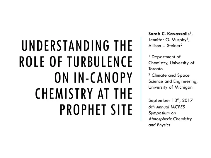
Trunk Space Crown Space Canopy Height (22.5m) Model domain height: 3-5km
29m 21m 13m 5m 34m
Kavassalis - IACPES 2017
10
FORCAsT (Ashworth et al., 2015) was constrained by PROPHET-AMOS observations and used to model the campaign chemistry. In FORCAsT, mass fluxes are calculated by solving the continuity equation: 𝜖𝑑 𝜖𝑢 = 𝜖 𝑨 𝐿𝐼 𝜖𝑑 𝜖𝑨 + 𝑇𝑑 + 𝐷 Where c is the mixing ratio of the species of interest, KH is the turbulence exchange coefficient, SC includes contributions from emissions, deposition, and advection, and C represents chemical production and loss.