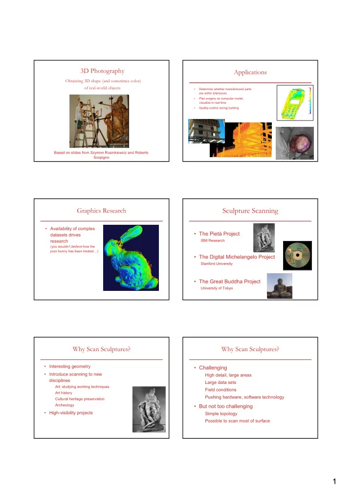
1 1 Issues Addressed The Digital Michelangelo Project Resolution - - PDF document

1 1

3D Photography

Obtaining 3D shape (and sometimes color)

• f real-world objects

Based on slides from Szymon Rusinkiewicz and Roberto Scopigno

Applications

• Determine whether manufactured parts

are within tolerances

• Plan surgery on computer model,

visualize in real time

• Quality control during building

Graphics Research

• Availability of complex

datasets drives research

(you wouldn’t believe how the poor bunny has been treated…)

Sculpture Scanning

• The Pietà Project

IBM Research

• The Digital Michelangelo Project

Stanford University

• The Great Buddha Project

University of Tokyo

Why Scan Sculptures?

• Interesting geometry
• Introduce scanning to new

disciplines

– Art: studying working techniques – Art history – Cultural heritage preservation – Archeology

• High-visibility projects

Why Scan Sculptures?

• Challenging

– High detail, large areas – Large data sets – Field conditions – Pushing hardware, software technology

• But not too challenging

– Simple topology – Possible to scan most of surface

2 2

Issues Addressed

• Resolution
• Coverage

– Theoretical: limits of scanning technologies – Practical: physical access, time

• Type of data

– High-res 3D data vs. coarse 3D + normal maps – Influenced by eventual application

• Intellectual Property

The Digital Michelangelo Project Goals

• Scan 10 sculptures by Michelangelo
• High-resolution (“quarter-millimeter”)

geometry

• Side projects: architectural scanning

(Accademia and Medici chapel), scanning fragments of Forma Urbis Romae

Why Capture Chisel Marks?

Atlas Atlas

ugnetto ugnetto ugnetto

? ?

Why Capture Chisel Marks?

Day (Medici Chapel) Day (Medici Chapel) 2 mm 2 mm

Scanner Design

4 motorized axes 4 motorized axes laser, range camera, laser, range camera, white light, and color camera white light, and color camera

3 3

Scanning a Large Object

• Calibrated motions

– pitch (yellow) – pan (blue) – horizontal translation (orange)

• Uncalibrated motions

– vertical translation – rolling the gantry – remounting the scan head

Single Scan of St. Matthew

1 mm 1 mm 1 mm

Statistics About the Scan of David

• 480 individually aimed scans
• 0.3 mm sample spacing
• 2 billion polygons
• 7,000 color images
• 32 gigabytes
• 30 nights of scanning
• 22 people

Head of Michelangelo’s David

Photograph Photograph 1.0 mm computer model 1.0 mm computer model

Side project: The Forma Urbis Romae Forma Urbis Romae Fragment

side face

4 4

IBM’s Pietà Project

• Michelangelo’s

“Florentine Pietà”

• Late work (1550s)
• Partially destroyed by

Michelangelo, recreated by his student

• Currently in the Museo

dell’Opera del Duomo in Florence

Results The Great Buddha Project

• Great Buddha of

Kamakura

• Original made of wood,

completed 1243

• Covered in bronze and

gold leaf, 1267

• Approx. 15 m tall
• Goal: preservation of

cultural heritage

3D Scanning

The acquisition of a single range map is only an intermediate single step of the overall acquisition session

The 3D scanning pipeline

• 3D Scanning:

– Acquisition planning – Acquisition of multiple range maps – Range maps Editing – Registration of range maps – Merge of range maps – Mesh Editing – Geometry simplification – Capturing appearance – Archival and data conversion

5 5

Acquisition Planning

Selecting the set of views is not easy

Acquisition Planning

Definition of the optimal acquisition patchwork:

• Given: scanner & object characteristics
• Obtain an optimal & complete coverage (all object

surface covered): – Minimal number of scans – Sufficient inter-scan overlap (registration) – Where each scan should be:

• shot from a view direction nearly orthogonal to the

surface

• physically feasible (consider potential collisions with the
• bject/environment, self-occlusions)
• NP-hard problem find good heuristics & approximate

solutions NP-hard problem find good heuristics & approximate solutions

Registration and Merging

First: Register all range maps Second: Merge in a single triangulated surface with no redundancy

Registration

• Independent scans are

defined in coordinate spaces which depend on the spatial locations of the scanning unit and the object at acquisition time. They have to be registered (roto- translation) to lie in the same space

• Standard approach:
• 1. initial manual placement
• 2. Iterative Closest Point

(ICP) [Besl92,CheMed92]

Manuel Pairwise Registration

Mode 1) The user manually places a range map over another (interactive manipulation) Mode 2) Selection

• f multiple pairs of

matching points

Pairwise Registration

• An approximation to the

distance between range scans is: –

E = S || T qi – pi ||2

• where the qi are samples

from scan Q and the pi are the corresponding points of scan P.

6 6

Iterative Closet Point (ICP) [Besl+92]

• If the correspondences are known a priori,

then there is a closed form solution for T. However, the correspondences are not known in advance.

• Iterative closest point (ICP) [Besl+92]

– Start from an approximate registration – Repeat

• Identify corresponding points

(minimal distance)

• Compute and apply the optimal rigid

motion T

– Until registration error E is small

Registration, many more issues

Pairwise Sequential vs. Global [Pulli99] Using Color in registration [Bernardini00]

Image by F. Bernardini

So far…

• Mainly engineering problems,

planning, scanning and registration.

• Now, once registered, all scans

have to be fused in a single, continuous, hole-free mesh

• In other words – surface

reconstruction…

• Or, surface consolidation

Consolidation

Desirable properties for surface reconstruction:

– No restriction on topological type – Representation of range uncertainty – Utilization of all range data (integrate over overlapped regions) – Incremental and order independent updating – Time and space efficiency – Robustness (to noise) – Ability to fill holes in the reconstruction

Filling Holes [Sharf+04]

Holes… Smooth Interpolation Intelligent…

Filling Holes [Sharf+04]

7 7

Methods that construct triangle meshes directly:

Reconstruction from point clouds

• Local Delaunay triangulations [Boissonat84]
• Alpha shapes [Edelsbrunner+92]
• Crust algorithm [Amenta+98]
• Delaunay-based sculpturing [Attene+00]
• Ball Pivoting [Bernardini+99]
• Localized Delaunay [Gopi+00]

Reconstruction from range maps

• Re-triangulation in projection plane [Soucy+92]
• Zippering in 3D [Turk+94]

Methods that construct implicit functions:

• Signed distances to nearest surface [Hilton+96]
• Signed distances to sensor + space carving [Curless+96]
• Marching Intersections [Rocchini+00]

From range maps

• Voxel-based signed distance functions [Hoppe+92]
• Point Set Surfaces [Levin, Alexa, Flieshman+ 01]
• Radial Basis Functions [Carr+01]
• Partition of Unity [Ohtake+03]

From point clouds

Single Laser Range Image

A single scan is a grid: Connect adjacent samples when z-difference is small.

Range images

• Converting a range image into a range surface is easy.
• Use a tessellation threshold

Zippering [Turk+94]

• Redundancy removal and zippering

Image by Brian Curless, Sig’2000 Course Notes

So, what’s the problem?

scan, register, and apply some zippering?

8 8

Sampling quality and reconstruction issues

Ideal Sampling Uneven Sampling or holes?

Sampling quality and reconstruction issues

Interpolating? Or noisy sampling?

Sampling quality and reconstruction issues

Solid Object with thin section?

Sampling quality and reconstruction issues

Solid Object with small features?

Sampling quality and reconstruction issues

Smooth or Sharp features?

Methods that construct implicit functions:

• Signed distances to nearest surface [Hilton+96]
• Signed distances to sensor + space carving [Curless+96]
• Marching Intersections [Rocchini+00]

From range maps

• Voxel-based signed distance functions [Hoppe+92]
• Point Set Surfaces [Levin, Alexa, Flieshman+ 01]
• Radial Basis Functions [Carr+01]
• Partition of Unity [Ohtake+03]

From point clouds

9 9

Implicit Surface Representation

Represented as a function f(x,y,z) = 0 Volumetric representation One important implicit function is the distance function

Distance Field

• Define an implicit function D(p) = distance to the

surface at point p > 0 outside the surface < 0 inside the surface = 0 on the surface Use interpolation to compute distance at an arbitrary point

Distance Field Marching Cube Tangent plane and signed distance estimation

• Compute ni that

minimizes Where

( )

∑

⋅ −

j

p i i j

n x p

( )

i j

x Nbhd p ∈

Assume that if points are close then normals are nearly parallel

Results of Three Phases[Hoppe92]

Points Phase 1 Phase 2

Phase 3

10 10

Phase 1: Initial Surface Estimation

• From points to mesh:

–

Inferring topological type

–

Creating geometric approximation

Points (4,102) Initial Mesh (886 vertices)

Phase 2: Mesh optimization

Phase 1 (886 vertices) Phase2 (163 vertices)

• Input: data points P, initial mesh
• Output: optimized mesh M

Phase 2: Mesh Optimization

• Optimize the energy function:

Optimization rules use edge collapse and expand

• Sum of square distances

– (accurate)

• Number of vertices

– (sparse)

• Regulation term

– make vertices with equidistance

Optimization steps

Repeat (K’,V’)=GenerateLegalMove(K,V) V’ = OptVertexPosition(K’,V’) if E(K’,V’) < E(K,V) (K,V) = (K’, V’) endif Until converges

Phase 3: Piecewise Smooth Surface Piecewise smooth

• Not everywhere smooth, but piecewise

smooth! Smooth surface Piecewise smooth surface

11 11

Point Set Surfaces[Alexa+01]

• Smooth surface

manifold representation

• f point sets
• Up-sample
• Down-sample
• Noise reduction
• Interactive rendering

The moving least squares (MLS)[Levin]

Constructive definition of the surface:

• Input point r
• Compute a local reference plane Hr=<q,n>
• Compute a local polynomial over the plane Gr
• Project point r’=Gr(0)

r

Gr

Hr

q n

Reconstruction by Radial Bases Function

• Scattered data interpolation

scheme

• Input: set of points on the surface
• Output: Implicit function that

interpolates the points in a nice way

• Nice way:

ds s f s f s f f E

yy xy s xx

) ( ) ( 2 ) ( ) (

2 2 2

+ + = ∫

Ω ∈

ds s f ds s f ds s f s f s f s f f E

yz xz xy zz yy s xx

) ( 2 ) ( 2 ) ( 2 ) ( ) ( ) ( ) (

2 2 2 2 2 2

+ + + + + = ∫

Ω ∈

Form of solution

• The solution is of the form:
• Where P is a polynomial
• Φ is a radially symmetric

function

• The trivial solution is wi=0

( )

∑

=

− Φ =

n i i i

x x w x f

1

) (

Forming a signed-distance function Off surface points

• For every point, add two off-

surface points, one inside and

• ne outside the surface in the

direction of the normal

• Add a point only if it is closest

to its source

• N≈3n points

Forming a signed-distance function

• Off-surface points are projected along surface

normals Outward normal points On-surface points Inward normal points

12 12

Radial basis functions

Minimizes 2nd derivative in 3D Minimizes 2nd derivative in 2D

r r = Φ ) ( r r r log ) (

2

= Φ

3

) ( r r = Φ

Minimizes 3nd derivative in 3D

( )

∑

=

− Φ =

n i i i

x x w x f

1

) (

Computing the weights

• Input : {xi}, {fi}. Compute {wi}

( )

∑

=

− Φ =

n i i i

x x w x f

1

) (

( )( ) ( )

f W ANxN =

Unknowns to compute Function values Matrix dependent on the locations of the data points

Computing - example

• Symmetric positive matrix

( ) ( ) ( ) ( ) ( ) ( ) ( ) ( ) ( )

⎟ ⎟ ⎟ ⎟ ⎟ ⎟ ⎟ ⎟ ⎟ ⎠ ⎞ ⎜ ⎜ ⎜ ⎜ ⎜ ⎜ ⎜ ⎜ ⎜ ⎝ ⎛ = ⎟ ⎟ ⎟ ⎟ ⎟ ⎟ ⎟ ⎟ ⎟ ⎠ ⎞ ⎜ ⎜ ⎜ ⎜ ⎜ ⎜ ⎜ ⎜ ⎜ ⎝ ⎛ ⎟ ⎟ ⎟ ⎟ ⎟ ⎟ ⎟ ⎟ ⎟ ⎟ ⎠ ⎞ ⎜ ⎜ ⎜ ⎜ ⎜ ⎜ ⎜ ⎜ ⎜ ⎜ ⎝ ⎛ − Φ − Φ − Φ − Φ − Φ − Φ − Φ − Φ − Φ

N N N N N N N N

f f f W W W x x x x x x x x x x x x x x x x x x M M K M M K

2 1 2 1 2 1 2 2 2 2 1 1 1 2 1 1

Complexity

Straight-forward method:

• Storage O(N2)
• Solving the Wi O(N3)
• Evaluating f(x) O(N)

Fast method [Carr01]

• Storage O(N)
• Solving the Wi

O(NlogN)

• Evaluating f(x)

O(1) + O(NlogN) setup

Carr 01

Simplification (center reduction)

• Reduce the number of centers (points)
• Greedy algorithm, reduce points as long as the surface is

close enough

Carr 01

Why use implicit functions

• Well-defined interior and exterior
• Topology changes easy
• Constructive Solid Geometry
• Shape Interpolation

13 13

Multi-level Partition of Unity

Partition of unity Partition of unity

Large error region is subdivided

Support of Support of Q( Q(x x) ) (B (B-

• spline

spline) )

Q( Q(x x)=0 )=0 (quadric) (quadric)

∑ ∑

= ) ( ) ( ) ( ) ( x x x x

i i i

w Q w f

Weighted average of Weighted average of the local functions the local functions

f( f(x x)=0 )=0

Sharp Features

Ray Ray-

• traced

traced f=0 f=0

Corner Corner function function Edge Edge function function Standard Standard quadric quadric

Piecewise quadric Piecewise quadric functions functions

Local analysis of Local analysis of points and normals points and normals

The moving least squares (MLS)[Levin]

Constructive definition of the surface:

• Input point r
• Compute a local reference plane Hr=<q,n>
• Compute a local polynomial over the plane Gr
• Project point r’=Gr(0)

r

Gr

Hr

q n

Local reference plane

• Plane equation: Hr=<q,n>
• Hr=min Σi(d(xi,Hr)θ(||q- xi||)

Non-linear optimization Where

• {xi} neighbor points

฀ θ(x)=exp(-x2/h2)

• h reconstruction parameter,

depends on the spacing of points

• Note: q != r

Hr r

Gr

Hr

q n

Projecting the point

• Gr=min Σi|G(xi,x)-xi,y|θ(||q- xi||)

Linear optimization

• r’=Gr(0)

r

Gr

Hr

q n

Noise Reduction

• Using high values of h

– Smoother surfaces – Less detail

14 14

Up sample

• Create a local

Voronoi diagram

• Add points at Voronoi

vertex with the largest radius

• Stop when spacing is

small enough

Downsample

• Sp- Surface
• Remove Point pi if |Sp-SP-pi|<ε
• Speedup: Evaluate |pi-Project(pi, SP-pi)|