0 1 0 0 0 0 0 1 1 0 0 0 0 0 2 2 1 1 - - PDF document

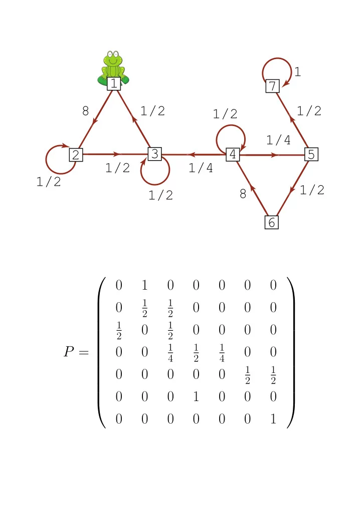
8 8 1/2 1/2 1/2 1/2 1 1/2 1/4 1/2 1/2 1/4 4 3 7 6 1 2 5 P =              1

1 2 1 2 1 2 1 2 1 4 1 2 1 4 1 2 1 2

1 1             

Andrei Andreevich Markov (1856–1922)

In Example 1.1 P (n) =              1

1 2 1 2 1 2 1 2 1 4 1 2 1 4 1 2 1 2

1 1             

n

→             

1 5 2 5 2 5 1 5 2 5 2 5 1 5 2 5 2 5 2 15 4 15 4 15 1 3 1 15 2 15 2 15 2 3 2 15 4 15 4 15 1 3

1             

Find the classes in P and say whether they are open

• r closed.

P =          

1 2 1 2

1

1 3 1 3 1 3 1 2 1 2

1 1          

1 2 3 4 5 6

Engel’s probabilistic abacus Consider an absorbing Markov chain with rational transition probabilites, as in P =       

1 2 1 4 1 4 1 3 1 3 1 3 1 3 2 3

1 1        Clearly {1, 2, 3} are transient and {4, 5} are absorbing. Suppose we want to find h1 (= α14), the probability that starting in state 1 absorption takes place in state

• 4. The usual method is to solve the RHE:

h1 = 1

2h1 + 1 4h2 + 1 4h3

h2 = 1

3h1 + 1 3h3 + 1 3h4

h3 = 1

3h3 + 2 3h5

h4 = 1 h5 = 0 Alternatively, we can use Engel’s algorithm, or playing a so-called chip firing game.

We create one node for each state and put some chips (or tokens) at the nodes corresponding to the non-absorbing states, {1, 2, 3}. Suppose that there are integers ri, ri1, . . . , rin such that pij = rij/ri for all j. If there were ri chips at node i we could ‘fire’ or ‘make a move’ in node i. This means taking ri chips from node i and moving rij of them to node j, for each j.

1/2 1/4 1/4 1/3 1/3 1/3 1/3 2/3

The critical loading is one in which each node has one less chip that it needs to fire, i.e. ci = ri −1. So c1 = 3 and c2 = c3 = 2. We start with a critical loading by placing tokens at nodes 1, 2, 3, 4, 5 in numbers: (3, 2, 2, 0, 0), and add a large number of tokens to another node 0.

‘Firing’ node 0 means moving one token from node 0 to node 1. Engel’s algorithm also imposes the rule that node 0 may be fired only if no other node can fire. Starting from the critical loading we fire node 0 and then node 1: (3, 2, 2, 0, 0) → (4, 2, 2, 0, 0)

1

→ (2, 3, 3, 0, 0)

1/2 1/4 1/4 1/3 1/3 1/3 1/3 2/3 1/2 1/4 1/4 1/3 1/3 1/3 1/3 2/3 1/2 1/4 1/4 1/3 1/3 1/3 1/3 2/3

Now nodes 2 or 3 could fire. Suppose we fire 3, then 2: (2, 3, 3, 0, 0)

3

→ (2, 3, 1, 0, 2)

2

→ (3, 0, 2, 1, 2)

1/2 1/4 1/4 1/3 1/3 1/3 1/3 2/3

The same loading would be reached if we had fired 2 and then 3. This fact is important! Now we fire the sequence 0, 1, 3, 0, 0, 1, 0: (3, 0, 2, 1, 2) → (4, 0, 2, 1, 2)

1

→ (2, 1, 3, 1, 2)

3

→ (2, 1, 1, 1, 4) → (3, 1, 1, 1, 4) → (4, 1, 1, 1, 4)

1

→ (2, 2, 2, 1, 4) → (3, 2, 2, 1, 4) which leaves us at

1/2 1/4 1/4 1/3 1/3 1/3 1/3 2/3

At this point we stop, because nodes 1, 2 and 3 now have exactly the same loading as at the start. We are at (3, 2, 2, 0, 0) + (0, 0, 0, 1, 4). We have fired 0 five times and ended up back at the critical loading, but with 1 token in node 4 and 4 tokens in node 5. Thus h1 = 1/5.

Why does this algorithm work? It is fairly obvious that if the initially critically loaded configuration of the transient states reoccurs then the numbers of tokens that have appeared in the nodes that correspond to the absorbing states must be in quantities that are in pro- portion to the absorptions probabilities, α1j. But why is the initial critically loaded configuration guaranteed to eventually reappear? This puzzled Engel in 1976, and was proved circa 1979 by Peter Doyle, whose proof is in Appendix C. The proof is interesting. There is, in fact, a rich literature on the properties

• f chip firing games and this proof generalises to show

that many chip firing games have the property that the termination state does not depend on the order in which moves are made.

X Y Z

Feasibility of wind instruments Lord Rayleigh in “On the theory of resonance” (1899) proposed a model for wind instruments in which the creation of resonance through a vibrating column of air requires repeated expansion and contraction of a mass of air at the mouth of the instrument, air being modelled as an incompressible fluid. Think instead about an infinite rectangular lattice

• f cities. City (0,0) wishes to expand its tax base and

does this by inducing a business from a neighboring city to rellocate to it. The impoverished city does the same (choosing to “beggar-its-neighbour” randomly amongst its 4 neighbours since “beggars can’t be choosers”), and this continues, just like a 2-D random walk. Unfortu- nately, this means that with probability 1 the walk re- turns to the origin city who eventually finds that one of its own businesses is induced away by one of its neigh- bours, leaving it no better off than at the start. We might say that it is “infinitely-hard to expand the tax base by a beggar-your-neighbour policy”. However, in 3-D there is a positive probability (about 0.66) that the city (0, 0) will never be beggared by one of its 6 neighbours.

By analogy, we see that in 2-D it will be “infinitely hard” to expand the air at the mouth of the wind in- strument, but in 3-D the energy required is finite. That is why Doyle and Snell say wind instruments are possi- ble in our 3-dimensional world, but not in Flatland. We will learn in Lecture 12 something more about the method that Rayleigh used to show that the energy required to create a vibrating column of air in 3-D is finite.

Invariant distribution of a two-state chain

1 2 a 1-a 1-b b

P = 1 − α α β 1 − β

• P n =
• β

α+β + α α+β(1 − α − β)n α α+β − α α+β(1 − α − β)n β α+β − β α+β(1 − α − β)n α α+β + β α+β(1 − α − β)n

• →
• β

α+β α α+β β α+β α α+β

• =

π1 π2 π1 π2

P = (0.85)

              

1 2 1 2

1

1 2 1 2 1 3 1 3 1 3 1 3 1 3 1 3

1

1 3 1 3 1 3 1 2 1 2

               + (0.15)1 8                1 1 1 1 1 1 1 1 1 1 1 1 1 1 1 1 1 1 1 1 1 1 1 1 1 1 1 1 1 1 1 1 1 1 1 1 1 1 1 1 1 1 1 1 1 1 1 1 1 1 1 1 1 1 1 1 1 1 1 1 1 1 1 1               

P 10 =

           0.065 0.092 0.045 0.098 0.11 0.18 0.15 0.26 0.060 0.094 0.047 0.095 0.11 0.19 0.17 0.24 0.064 0.092 0.045 0.098 0.11 0.18 0.15 0.26 0.066 0.091 0.044 0.099 0.11 0.18 0.15 0.26 0.065 0.092 0.045 0.098 0.11 0.18 0.15 0.26 0.057 0.095 0.049 0.095 0.10 0.20 0.17 0.23 0.060 0.094 0.047 0.096 0.11 0.19 0.16 0.24 0.068 0.090 0.043 0.10 0.12 0.17 0.14 0.27           

P 20 =

           0.063 0.093 0.046 0.097 0.11 0.18 0.16 0.25 0.063 0.093 0.046 0.097 0.11 0.18 0.16 0.25 0.063 0.093 0.046 0.097 0.11 0.18 0.16 0.25 0.063 0.093 0.046 0.097 0.11 0.18 0.16 0.25 0.063 0.093 0.046 0.097 0.11 0.18 0.16 0.25 0.063 0.093 0.046 0.097 0.11 0.18 0.16 0.25 0.063 0.093 0.046 0.097 0.11 0.18 0.16 0.25 0.063 0.093 0.046 0.097 0.11 0.18 0.16 0.25           

Theorem 5.8. Suppose P is irreducible and recurrent. Then for all j ∈ I we have P(Tj < ∞) = 1. Theorem 8.3. Suppose P is irreducible and λ ≥ 0 and λ = λP. Then λ ≡ 0 or (0 < λi < ∞ for all i) or λ ≡ ∞. Theorem 8.4 (Existence of an invariant measure). Let P be irreducible and recurrent. Then (i) γk

k = 1.

(ii) γk = (γk

i : i ∈ I) satisfies γkP = γk.

(iii) 0 < γk

i < 1 for all i.

Theorem 8.5 (Uniqueness of an invariant measure). Let P be irreducible and let λ be an invariant measure for P with λk = 1. Then λ ≥ γk. If in addition P is recurrent, then λ = γk. Theorem 9.1. Let P be irreducible. Then the following are equivalent: (i) every state is positive recurrent; (ii) some state i is positive recurrent; (iii) P has an invariant distribution, π say. Moreover, when (iii) holds we have mi = 1/πi for all i.

A quotation from J. Michael Steele Coupling is one of the most powerful

• f the “genuinely probabilistic” techniques.

Here by “genuinely probabilistic” we mean something that works directly with random variables rather than with their analytical co-travelers (like distributions, densities, or characteristic functions).

Theorem 10.1 (Strong law of large numbers). Let Y1, Y2 . . . be a sequence of independent and identically distributed non-negative random variables with E(Yi) = µ. Then P Y1 + · · · + Yn n → µ as n → ∞

• = 1.

P =      

1 2 1 4 1 4 1 4 0 1 2 1 4 1 4 1 4 0 1 2 1 2 1 4 1 4 0

     

• p(n)

11 ,p(n) 12 , p(n) 13 , p(n) 14

• =

                 1. 0. 0. 0. 0. 0.5 0.25 0.25 0.3125 0.125 0.3125 0.25 0.234375 0.296875 0.203125 0.265625 0.257813 0.234375 0.273438 0.234375 0.244141 0.255859 0.240234 0.259766 0.253906 0.24707 0.253906 0.245117 0.247803 0.251709 0.248291 0.252197 0.251099 0.249023 0.250854 0.249023 0.249481 0.250519 0.249542 0.250458                  −

• i

p(n)

1i log2

• p(n)

1i

• =

                 0. 1.5 1.92379 1.98583 1.99685 1.99925 1.99982 1.99996 1.99999 2.                 

A random knight makes each permissible move with equal probability. If it starts in a corner, how long on average will it take to return?

2 3 3 4 4 4 6 6 6 8 8 8 8 6 4 4

The following chart shows {Xn}500

n=300 in a simulation of an

urn with 20 balls, started at X0 = 10. Below it the data is shown reversed. There is no apparent difference.

50 100 150 200 5 10 15 20 50 100 150 200 5 10 15 20

+

a a

v(a)=1

b b x x y y L L

v(b)=0

Probability and Measure

• Concepts such as ‘expectation’, ‘measure’, ‘strong

law of large numbers’ are developed rigorously.

• Limits are a key theme.

E.g. Pi(Xn makes infinitely many returns to i). This can takes only values 0 or 1 (never 1/2).

• Important

for many mathematicians, not just those who are specializing in

• ptimiza-

tion/probability/statistics. Typical question Let Ω = {0, 1}, F = B((0, 1)) be the Borel σ-field and let P be Lebesgue measure on (Ω, F). Give an example

• f an ergodic measure-preserving map θ : Ω → Ω.

Applied Probability

• Applications in queueing, communication networks,

insurance ruin, and epidemics.

• Stochastic processes in continuous time.
• Imagine our frog in Example 1.1 waits for an expo-

nentially distributed time before hopping to a new lily pad. What now is p57(t), t ≥ 0? As you might guess, we find this by solving differential equations, in place

• f the recurrence relations we had in discrete time.

Typical question Consider an M/G/r/0 loss system with arrival rate λ and service-time distribution F. Thus, arrivals form a Poisson process of rate λ, service times are independent with common distribution F, there are r servers and there is no space for waiting. Use Little’s Lemma to obtain a relation between the long-run average occupancy L and the stationary prob- ability π that the system is full.

Optimization and Control

• Add to Markov chains notions of cost, reward, and
• ptimization.
• Suppose we can pick, as a function of the current

state x, the transition matrix P, to be one of a set

• f k possible matrices, say P(a), a ∈ {ak, . . . , ak}.
• Perhaps we would like to steer our frog to arrive at

some particular lily pad in the least possible time,

• r with the least cost.
• Suppose three frogs are placed at different vertices
• f Z2. At each step we can choose one of the frogs

to make a random hop to one of its neighbouring

• vertices. We wish to minimize the expected time

until we first have a frog at the origin. This is like ‘playing golf with more than one ball’. Typical question In a television game show a contestant is successively asked questions Q1, . . . , Q9. After correctly answering Qi and hearing Qi+1 she has the option of either going home with 2i pounds or attempting to answer Qi+1. If she answers Qi+1 incorrectly then she goes home with

• nothing. If she answers Q9 correctly then the game ends

and she takes home 29 pounds.

Stochastic Financial Models

• Random walks, Brownian motion, Poisson process,

and other stochastic models that are useful in mod- elling financial products.

• Suppose our frog starts in state i and does a biased

random walk on {0, 1, . . . , 10}, eventually hitting state 0 or 10, where she then wins a prize worth £0

• r £10.

How much would we be willing to pay at time 0 for the right (option) to buy her final prize for £s? Typical question In a standard Black-Scholes model, the price at time t

• f a share is represented as St = exp(Xt). You hold a

perpetual American put option on this share, with strike K; you may exercise at any stopping time τ, and upon exercise you receive max{0, K−Sτ}. Let 0 < a < log K. Suppose you plan to use the exercise policy: ‘Exercise as soon as the price falls to ea or lower.’ Calculate what the option would be worth if you were to follow this policy.