What you should know after day 6 An introduction to WS 2018/2019 - - PDF document

An introduction to WS 2018/2019

• Dr. Sonja Grath
• Dr. Eliza Argyridou

Special thanks to:

• Dr. Benedikt Holtmann for sharing slides for this lecture

Data visualization and graphics

2

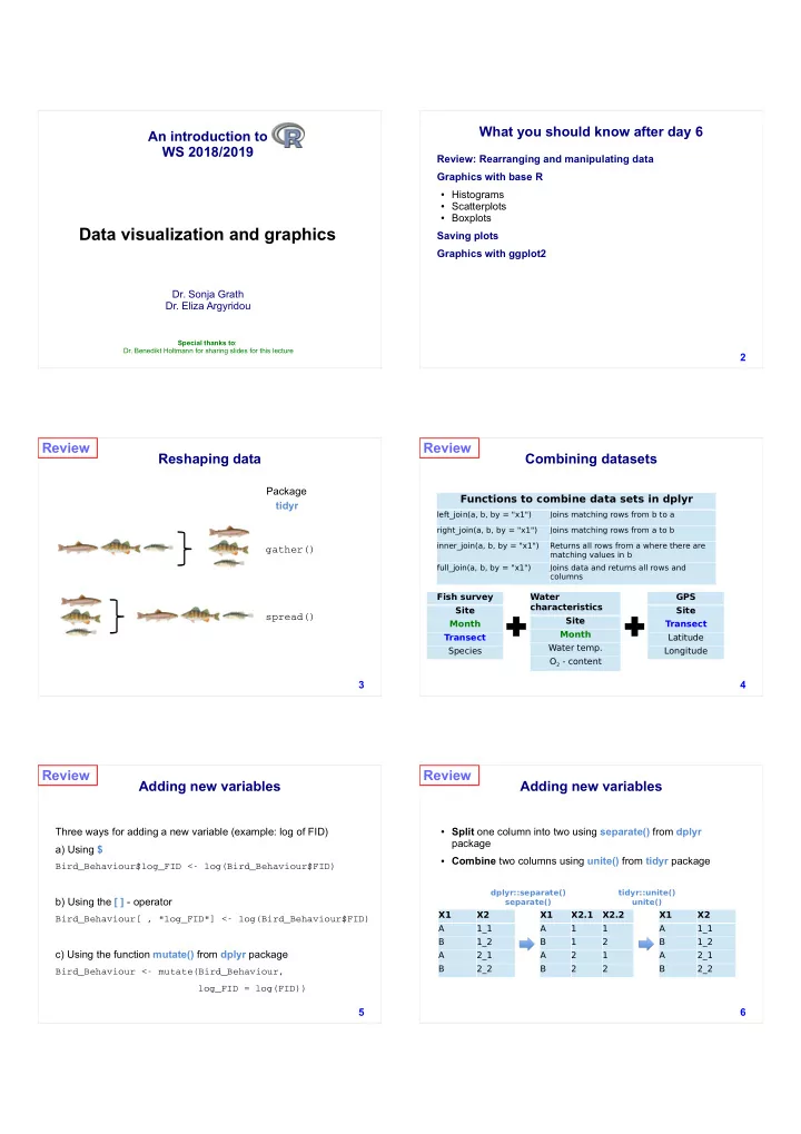
What you should know after day 6

Review: Rearranging and manipulating data Graphics with base R

• Histograms
• Scatterplots
• Boxplots

Saving plots Graphics with ggplot2 3

Reshaping data Review

Package tidyr gather() spread() 4

Combining datasets Review

Fish survey Site Month Transect Species Water characteristics Site Month Water temp. O2 - content GPS Site Transect Latitude Longitude

Functions to combine data sets in dplyr

left_join(a, b, by = "x1") Joins matching rows from b to a right_join(a, b, by = "x1") Joins matching rows from a to b inner_join(a, b, by = "x1") Returns all rows from a where there are matching values in b full_join(a, b, by = "x1") Joins data and returns all rows and columns

5

Adding new variables

Three ways for adding a new variable (example: log of FID) a) Using $

Bird_Behaviour$log_FID <- log(Bird_Behaviour$FID)

b) Using the [ ] - operator

Bird_Behaviour[ , "log_FID"] <- log(Bird_Behaviour$FID)

c) Using the function mutate() from dplyr package

Bird_Behaviour <- mutate(Bird_Behaviour, log_FID = log(FID))

Review

6

Adding new variables

• Split one column into two using separate() from dplyr

package

• Combine two columns using unite() from tidyr package

X1 X2 A 1_1 B 1_2 A 2_1 B 2_2 X1 X2.1 X2.2 A 1 1 B 1 2 A 2 1 B 2 2 X1 X2 A 1_1 B 1_2 A 2_1 B 2_2

dplyr::separate() separate() tidyr::unite() unite()

Review

7

Subsetting data

Subsetting data:

• Using [ ] – operator
• Using subset()
• With functions from the dplyr package

# selects the rows 1 to 3 and

# columns 1 to 4 Bird_Behaviour[1:3, 1:4]

# selects all rows with males Bird_Behaviour[Bird_Behaviour$Sex == "male", ] # selects all rows that have a value of FID greater than 10 or less than 15. We keep only the IND, Sex and Year column subset(Bird_Behaviour, FID > 10 | FID < 15, select = c(Ind, Sex, Year))

Operator Description > greater than >= greater than or equal to < less than <= less than or equal to == equal to != not equal to x & y x and y x | y x or y

Review

8

Subsetting data

Subsetting data with functions from the dplyr package

• You can subset by rows using slice() and filter()
• You can subset by columns with select()

# selects rows 3-5 Bird_Behaviour.slice <- slice(Bird_Behaviour, 3:5) # selects rows that meet certain criteria Bird_Behaviour.filter <- filter(Bird_Behaviour, FID < 5) # selects the columns Ind, Sex, and Fledglings Bird_Behaviour_col <- select(Bird_Behaviour, Ind, Sex, Fledglings) # excludes the variable disturbance Bird_Behaviour_reduced <- select(Bird_Behaviour,

• Disturbance)

Review

9

Graphics with base R

Simple graphics using plotting functions in the graphics package

• Base R, installed by default
• Easy and quick to type
• Wide variety of functions

Function Description hist() Histograms plot() Scatterplots, etc. boxplot() Box- and whisker plots barplot() Bar- and column charts dotchart() Cleveland dot plots contour Contour of a surface (2D) pie() Circular pie chart …

10

Graphics with base R

Creating a histogram with hist() Example 1: hist(Sparrows$Tarsus)

Histogram of Sparr

• ws$T

arsus

S p a r r

• w

s $ T a r s u s F r e q u e n c y 1 9 2 0 2 1 2 2 2 3 2 4 2 5 5 1 1 5 2

11

Graphics with base R

Creating a histogram with hist() Example 2: Alter colour and the number of bins hist(Sparrows$Tarsus, col = "grey", breaks = 50)

Histogram

• f Sparrow

s$ Tarsus

S p a r r

• w

s $ T a r s u s F r e q u e n c y 1 9 2 2 1 2 2 2 3 2 4 2 5 1 2 3 4 5 6

12

Graphics with base R

Creating a histogram with hist() Example 3: Add density curve hist(Sparrows$Tarsus, col = "grey", breaks = 50, freq = FALSE)

Histogram

• f Sparrows$Tarsus

S p a r r

• w

s $ T a r s u s D e n s i t y 1 9 2 2 1 2 2 2 3 2 4 2 5 . . 2 . 4 . 6

13

Graphics with base R

Creating a histogram with hist() Example 3: Add density curve hist(Sparrows$Tarsus, col="grey", breaks = 50, freq = FALSE) lines(density(Sparrows$Tarsus), col = "blue", lwd = 2)

Hist

• gram
• f Sparrows$T

arsus

S p a r r

• w

s $ T a r s u s D e n s i t y 1 9 2 2 1 2 2 2 3 2 4 2 5 . . 2 . 4 . 6

14

Graphics with base R

Creating a histogram with hist() Example 4: Plot only males hist(Sparrows[Sparrows$Sex == "Male",]$Tarsus, col = "grey", breaks = 50)

Histogram

• f Sparrow

s[Sparrow s$ Se x = = "M ale", ]$ Tarsus

S p a r r

• w

s [ S p a r r

• w

s $ S e x = = " Ma l e " , ] $ T a r s u s F r e q u e n c y 2 2 1 2 2 2 3 2 4 2 5 1 0 2 0 3 0 4 0 5

15

Graphics with base R

Creating a scatterplot with plot()

➔ Relationship between two continuous variables

Example 1: plot(Sparrows$Wing, Sparrows$Tarsus)

5 5 6 6 5 1 9 2 2 1 2 2 2 3 2 4 2 5 S p a r r

• w

s $ Wi n g S p a r r

• w

s $ T a r s u s

16

Graphics with base R

Creating a scatterplot with plot() Example 2: Alter axis limits and shape of symbols plot(Sparrows$Tarsus, Sparrows$Wing, xlim = c(50, 70), pch = 15, col = "blue")

5 5 5 6 6 5 7 1 9 2 2 1 2 2 2 3 2 4 2 5 S p a r r

• w

s $ Wi n g S p a r r

• w

s $ T a r s u s

 Try yourself: ?pch 17

Graphics with base R

Creating a scatterplot with plot() Example 3: Alter the size of plotting symbols plot(Sparrows$Wing, Sparrows$Tarsus, xlim = c(50,70), cex = 1.5)

5 5 5 6 6 5 7 1 9 2 1 2 3 2 5 S p a r r

• w

s $ Wi n g S p a r r

• w

s $ T a r s u s

18

Graphics with base R

Creating line graphs with plot() Examples:

data("pressure") plot(pressure$temperature, pressure$pressure) plot(pressure$temperature, pressure$pressure, type = "l")

0 5 1 5 2 5 3 5 0 2 6 p r e s s u r e $ t e m p e r a t u r e p r e s s u r e $ p r e s s u r e 0 5 1 5 2 5 3 5 0 2 6 p r e s s u r e $ t e m p e r a t u r e p r e s s u r e $ p r e s s u r e

19

Graphics with base R

Use the type argument to specify the type of plot Possible types

"p" points "l" lines "b" points connected by lines "o" points overlaid by lines "h" vertical lines from points to the zero axis "s" steps "n" nothing, only the axes

20

Graphics with base R

Creating a boxplot with boxplot()

➔ Relationship between continuous and categorical variables

Example 1: boxplot(Wing ~ Sex, data = Sparrows)

F e m a l e M a l e 5 5 6 6 5

21

Graphics with base R

Example 2:

boxplot(Wing ~ Sex, data = Sparrows, xlab = 'Sex', # Adds label to x-axis ylab = 'Wing length (mm)', # Adds label to y-axis col=c("red", "blue"), # Adds colour ylim = c(50,70), # Changes axis limits main = "Boxplot")) # Adds title

F e m a l e M a l e 5 5 5 6 6 5 7 Boxplot S e x Wi n g l e n g t h ( m m )

22

Graphics with base R

Example 2: Multiple grouping variables boxplot(Wing ~ Sex + Species, data = Sparrows, xlab = ’Species and Sex', ylab = 'Wing length (mm)', col=c("red", "blue"), ylim = c(50,70), main = ""))

F e ma l e . S E S P M a l e . S E S P F e ma l e . S S T S M a l e . S S T S 5 5 5 6 6 5 7 S p e c i e s a n d S e x Wi n g l e n g t h ( m m )

23

Graphics with base R

Common parameters in graphics

main title of the plot xlab label of x-axis ylab label of y-axis xlim range/limits of x-axis ylim range/limits of y-axis col colour of the points, bars, etc. can be character string or hexadecimal colour (e.g. #RRGGBB) breaks number of bins pch shape of symbol cex size of symbols lty line type lwd line width

24

Multiple plots on one page

The par() function:

• comes with an extensive list of graphical parameters you can

change (see ?par)

• Some options are helpful; others you may never use

To plot multiple charts within the same window, you can use the mfcol or mfrow parameter For example, par(mfrow = c(2, 2) divides the graphic window into four panels (two rows and two columns)

25

Multiple plots on one page

H istogram

• f Spa

rrows$ Ta rsus S p a r r

• w

s $ T a r s u s D e n s i t y 1 9 2 0 2 1 2 2 2 3 2 4 2 5 . . 2 . 4 . 6 5 5 5 6 6 5 7 1 9 2 0 2 1 2 2 2 3 2 4 2 5 S p a r r

• w

s $ Wi n g S p a r r

• w

s $ T a r s u s F e m a l e Ma l e 5 5 5 6 6 5 7 Boxplot S e x Wi n g l e n g t h ( mm) F e m a l e . S E S P Ma l e . S S T S 5 5 5 6 6 5 7 S p e c i e s a n d S e x Wi n g l e n g t h ( mm) Histogra m

• f Spa

rrow s$ Ta rsus S p a r r

• w

s $ T a r s u s D e n s i t y 1 9 2 0 2 1 2 2 2 3 2 4 2 5 . . 2 . 4 . 6 5 5 5 6 6 5 7 1 9 2 0 2 1 2 2 2 3 2 4 2 5 S p a r r

• w

s $ Wi n g S p a r r

• w

s $ T a r s u s F e ma l e M a l e 5 5 5 6 6 5 7 Boxplot S e x Wi n g l e n g t h ( mm) F e ma l e . S E S P M a l e . S S T S 5 5 5 6 6 5 7 S p e c i e s a n d S e x Wi n g l e n g t h ( mm)

1 2 3 4 1 3 2 4

par(mfrow = c(2, 2)) par(mfcol = c(2, 2)) 26

Saving plots

There are several possibilities to save a plot

• 1. dev.print()

Example: plot(x, y, ….) # Make a plot # After you are finished with the plot use: dev.print(device = pdf, file = "filename.pdf") Important: When you are done, you have to close the printing device! dev.off() # shuts down current device 27

Saving plots

• 2. savePlot()

Example: plot(x, y, ….) # Make a plot savePlot(filename = "Figure1.pdf", type = "pdf") Important: It is possible that it does not work for your system! (uses X11 device, most Unix systems) 28

Saving plots

• 3. Plot directly into a fjle

Example:

# width and height are in inches per default pdf("Figure2.pdf", width = 4, height = 4) # You can execute multiple graphing commands hist(x) # The result of each will go into the pdf file plot(x, y, … ) dev.off()

But fjle is not printed on screen! 29

Different devices

Functions to save plots

pdf() Opens a pdf-fjle as device postscript() Opens a postscript-fjle as device png() Opens a png-fjle as device jpeg() Opens a jpeg-fjle as device tifg() Opens a tifg-fjle as device bmp() Opens a bmp-fjle as device

30

Graphics with ggplot2

Why use ggplot2?

• Many users, a lot of support
• Check out the ggplot2 documentation at http://docs.ggplot2.org/
• Very flexible and powerful
• Sophisticated plots for publication

31

Graphics with ggplot2

To create a plot you use the ggplot() function Basic structure:

ggplot(data, # data frame with variables to plot aes(x variable, y variable)) + # aestethics specifies which # variables to plot geom_object() # specifies the geometric objects

Commonly used geometric objects: Histogram: + geom_histogram() Scatterplot: + geom_point() Boxplot: + geom_boxplot() 32

Graphics with ggplot2

Creating a histogram with ggplot() Example:

ggplot(Sparrows, aes(Tarsus)) + geom_histogram(col = "grey", binwidth = 0.1) + xlab("Tarsus length (mm)") + ylab("Frequency")

2 4 6 2 2 2 2 4 T a r s u s l e n g t h ( m m ) F r e q u e n c y

33

Graphics with ggplot2

Creating a scatterplot with ggplot() Example 1: ggplot(Sparrows, aes(x = Wing, y = Tarsus)) + geom_point()

2 2 2 2 4 5 5 6 6 5

S p a r r

• w

s $ Wi n g S p a r r

• w

s $ T a r s u s

34

Graphics with ggplot2

Creating a scatterplot with ggplot() Example 2: Avoid overplotting of symbols ggplot(Sparrows, aes(x = Wing, y = Tarsus))+ geom_point(position=position_jitter(width=0.5, height=0)) 35

Graphics with ggplot2

Creating a scatterplot with ggplot() Example 2: Avoid overplotting of symbols

2 2 2 2 4 5 5 6 6 5 Wi n g T a r s u s

36

Graphics with ggplot2

Creating a scatterplot with ggplot() Example 3: Alter colour, shape, and size of symbols ggplot(Sparrows, aes(x = Wing, y = Tarsus, colour = Sex, shape = Species)) + geom_point(size = 2)

37

Graphics with ggplot2

Creating a scatterplot with ggplot() Example 3: Alter colour, shape, and size of symbols

2 2 2 2 4 5 5 6 6 5

Wi n g T a r s u s S p e c i e s

S E S P S S T S

S e x

F e m a l e M a l e

38

Graphics with ggplot2

Creating a boxplot with ggplot() Example 1:

ggplot(Sparrows, aes(Sex, Wing, fill = Sex)) + geom_boxplot()

5 5 6 6 5 F e ma l e M a l e

S e x Wi n g S e x

F e ma l e Ma l e

Wait... where do the colours come from???

ggplot2 uses default values for the colours, see for example:

myPlot <- ggplot(Sparrows, aes(Sex, Wing, fill = Sex)) + geom_boxplot() ggplot_build(myPlot)$data ... fill: #F8766D, #00BFC4

39

Saving a ggplot

Save a plot from ggplot2 with print() Example 1: print a ggplot to a file # Print the plot to a pdf file data("mtcars") pdf("myplot.pdf") myplot <- ggplot(mtcars, aes(wt, mpg)) + geom_point() print(myplot) dev.off() 40

Saving a ggplot

Save a plot from ggplot2 with ggsave() Example 2: save the last ggplot # 1. Create a plot # The plot is displayed on the screen ggplot(mtcars, aes(wt, mpg)) + geom_point() # 2. Save the plot to a pdf ggsave("myplot.pdf") 41

Graphics with ggplot2

Preparing plots for publication

• Title and axis labels
• Range of axes
• Colours
• Overall appearance (themes)
• Text size
• Legend

42

Graphics with ggplot2

Preparing plots for publication

• Title and axis labels
• Range of axes
• Colours
• Overall appearance (themes)
• Text size
• Legend

5 5 5 6 6 5 7 F e m a l e M a l e

S e x Wi n g l e n g t h ( m m)

S p a r r

• w

m

• r

p h

• l
• g

y

43

Further reading

http://www.cookbook-r.com/ http://www.cookbook-r.com/Graphs/ http://docs.ggplot2.org/ http://r4ds.had.co.nz/