w o o o o o o o x o o o x o o o that represents how - - PowerPoint PPT Presentation

IAML: Logistic Regression

Nigel Goddard School of Informatics Semester 1

1 / 22

Outline

◮ Logistic function ◮ Logistic regression ◮ Learning logistic regression ◮ Optimization ◮ The power of non-linear basis functions ◮ Least-squares classification ◮ Generative and discriminative models ◮ Relationships to Generative Models ◮ Multiclass classification ◮ Reading: W & F §4.6 (but pairwise classification,

perceptron learning rule, Winnow are not required)

2 / 22

Decision Boundaries

◮ In this class we will discuss linear classifiers. ◮ For each class, there is a region of feature space in which

the classifier selects one class over the other.

◮ The decision boundary is the boundary of this region. (i.e.,

where the two classes are “tied”)

◮ In linear classifiers the decision boundary is a line.

3 / 22

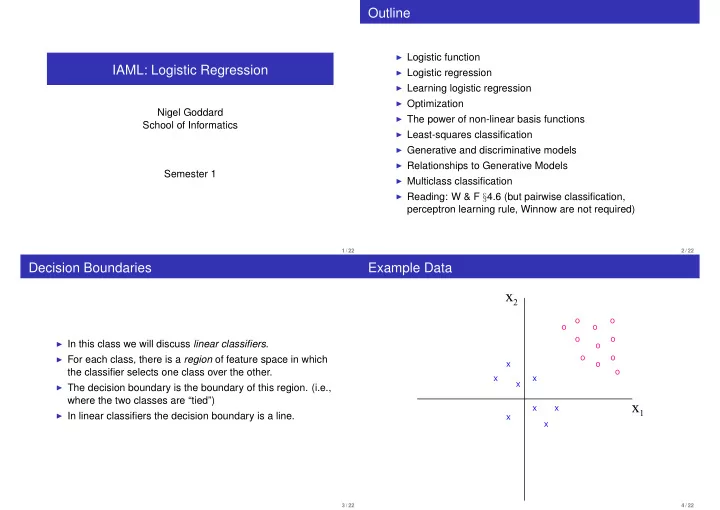
Example Data

x x x x x x x x

• x1

x2

4 / 22

Linear Classifiers

x x x x x x x x

• x1

x2 ◮ In a two-class linear classifier, we

learn a function F(x, w) = w⊤x + w0 that represents how aligned the instance is with y = 1.

◮ w are parameters of the classifier

that we learn from data.

◮ To do classification of an input x:

x → (y = 1) if F(x, w) > 0

5 / 22

A Geometric View

x x x x x x x x

• x1

x2 w

6 / 22

Explanation of Geometric View

◮ The decision boundary in this case is

{x|w⊤x + w0 = 0}

◮ w is a normal vector to this surface ◮ (Remember how lines can be written in terms of their

normal vector.)

◮ Notice that in more than 2 dimensions, this boundary will

be a hyperplane.

7 / 22

Two Class Discrimination

◮ For now consider a two class case: y ∈ {0, 1}. ◮ From now on we’ll write x = (1, x1, x2, . . . xd) and

w = (w0, w1, . . . wd).

◮ We will want a linear, probabilistic model. We could try

P(y = 1|x) = w⊤x. But this is stupid.

◮ Instead what we will do is

P(y = 1|x) = f(w⊤x)

◮ f must be between 0 and 1. It will squash the real line into

[0, 1]

◮ Furthermore the fact that probabilities sum to one means

P(y = 0|x) = 1 − f(w⊤x)

8 / 22

The logistic function

◮ We need a function that returns probabilities (i.e. stays

between 0 and 1).

◮ The logistic function provides this ◮ f(z) = σ(z) ≡ 1/(1 + exp(−z)). ◮ As z goes from −∞ to ∞, so f goes from 0 to 1, a

“squashing function”

◮ It has a “sigmoid” shape (i.e. S-like shape)

−6 −4 −2 2 4 6 0.1 0.2 0.3 0.4 0.5 0.6 0.7 0.8 0.9

9 / 22

Linear weights

◮ Linear weights + logistic squashing function == logistic

regression.

◮ We model the class probabilities as

p(y = 1|x) = σ(

D

• j=0

wjxj) = σ(wTx)

◮ σ(z) = 0.5 when z = 0. Hence the decision boundary is

given by wTx = 0.

◮ Decision boundary is a M − 1 hyperplane for a M

dimensional problem.

10 / 22

Logistic regression

◮ For this slide write ˜

w = (w1, w2, . . . wd) (i.e., exclude the bias w0)

◮ The bias parameter w0 shifts the position of the

hyperplane, but does not alter the angle

◮ The direction of the vector ˜

w affects the angle of the

• hyperplane. The hyperplane is perpendicular to ˜

w

◮ The magnitude of the vector ˜

w effects how certain the classifications are

◮ For small ˜

w most of the probabilities within the region of the decision boundary will be near to 0.5.

◮ For large ˜

w probabilities in the same region will be close to 1 or 0.

11 / 22

Learning Logistic Regression

◮ Want to set the parameters w using training data. ◮ As before:

◮ Write out the model and hence the likelihood ◮ Find the derivatives of the log likelihood w.r.t the

parameters.

◮ Adjust the parameters to maximize the log likelihood. 12 / 22

◮ Assume data is independent and identically distributed. ◮ Call the data set D = {(x1, y1), (x2, y2), . . . (xn, yn)} ◮ The likelihood is

p(D|w) =

n

• i=1

p(y = yi|xi, w) =

n

• i=1

p(y = 1|xi, w)yi (1 − p(y = 1|xi, w))1−yi

◮ Hence the log likelihood L(w) = log p(D|w) is given by

L(w) =

n

• i=1

yi log σ(w⊤xi) + (1 − yi) log(1 − σ(w⊤xi))

13 / 22

◮ It turns out that the likelihood has a unique optimum (given

sufficient training examples). It is convex.

◮ How to maximize? Take gradient

∂L ∂wj =

n

• i=1

(yi − σ(wTxi))xij

◮ (Aside: something similar holds for linear regression

∂E ∂wj =

n

• i=1

(wTφ(xi) − yi)xij where E is squared error.)

◮ Unfortunately, you cannot maximize L(w) explicitly as for

linear regression. You need to use a numerical

• ptimisation method, see later.

14 / 22

Fitting this into the general structure for learning algorithms:

◮ Define the task: classification, discriminative ◮ Decide on the model structure: logistic regression model ◮ Decide on the score function: log likelihood ◮ Decide on optimization/search method to optimize the

score function: numerical optimization routine. Note we have several choices here (stochastic gradient descent, conjugate gradient, BFGS).

15 / 22

XOR and Linear Separability

◮ A problem is linearly separable if we can find weights so

that

◮ ˜

wTx + w0 > 0 for all positive cases (where y = 1), and

◮ ˜

wTx + w0 ≤ 0 for all negative cases (where y = 0)

◮ XOR ◮ XOR becomes linearly separable if we apply a non-linear

tranformation φ(x) of the input — what is one?

16 / 22

The power of non-linear basis functions

x1 x2 −1 1 −1 1 φ1 φ2 0.5 1 0.5 1

Using two Gaussian basis functions φ1(x) and φ2(x)

Figure credit: Chris Bishop, PRML

As for linear regression, we can transform the input space if we want x → φ(x)

17 / 22

Generative and Discriminative Models

◮ Notice that we have done something very different here

than with naive Bayes.

◮ Naive Bayes: Modelled how a class “generated” the

feature vector p(x|y). Then could classify using p(y|x) ∝ p(x|y)p(y) . This called is a generative approach.

◮ Logistic regression: Model p(y|x) directly. This is a

discriminative approach.

◮ Discriminative advantage: Why spend effort modelling

p(x)? Seems a waste, we’re always given it as input.

◮ Generative advantage: Can be good with missing data

(remember how naive Bayes handles missing data). Also good for detecting outliers. Or, sometimes you really do want to generate the input.

18 / 22

Generative Classifiers can be Linear Too

Two scenarios where naive Bayes gives you a linear classifier.

• 1. Gaussian data with equal covariance. If

p(x|y = 1) ∼ N(µ1, Σ) and p(x|y = 0) ∼ N(µ2, Σ) then p(y = 1|x) = σ(˜ wTx + w0) for some (w0, ˜ w) that depends on µ1, µ2, Σ and the class priors

• 2. Binary data. Let each component xj be a Bernoulli variable

i.e. xj ∈ {0, 1}. Then a Na¨ ıve Bayes classifier has the form p(y = 1|x) = σ(˜ wTx + w0)

• 3. Exercise for keeners: prove these two results

19 / 22

Multiclass classification

◮ Create a different weight vector wk for each class, to

classify into k and not-k.

◮ Then use the “softmax” function

p(y = k|x) = exp(wT

k x)

C

j=1 exp(wT j x) ◮ Note that 0 ≤ p(y = k|x) ≤ 1 and C j=1 p(y = j|x) = 1 ◮ This is the natural generalization of logistic regression to

more than 2 classes.

20 / 22

Least-squares classification

◮ Logistic regression is more complicated algorithmically

than linear regression

◮ Why not just use linear regression with 0/1 targets?

−4 −2 2 4 6 8 −8 −6 −4 −2 2 4 −4 −2 2 4 6 8 −8 −6 −4 −2 2 4

Green: logistic regression; magenta, least-squares regression

Figure credit: Chris Bishop, PRML 21 / 22

Summary

◮ The logistic function, logistic regression ◮ Hyperplane decision boundary ◮ Linear separability ◮ We still need to know how to compute the maximum of the

log likelihood. Coming soon!

22 / 22