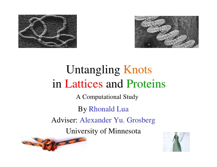
SLIDE 1
Untangling Knots in Lattices and Proteins
By Rhonald Lua Adviser: Alexander Yu. Grosberg University of Minnesota
A Computational Study
SLIDE 2 Human Hemoglobin (oxygen transport protein)
Globular proteins have dense, crystal-like packing density. Proteins are small biomolecular “machines” responsible for carrying out many life processes. (Structure by
M.F. PERUTZ)
SLIDE 3
Hemoglobin Protein Backbone (string of α−carbon units)
“ball of yarn” One chain
SLIDE 4 4x4x4 Compact Lattice Loop
Possible cube dimensions: 2x2x2,4x4x4,6x6x6,…,LxLxL,…
N e z )
(
1 −
- No. of distinct conformations:
(Flory)
z = 6 in 3D
SLIDE 5 Hamiltonian Path Generation
(A. Borovinskiy, based on work by R. Ramakrishnan, J.F. Pekny, J.M. Caruthers)
SLIDE 6
14x14x14 Compact Lattice Loop
SLIDE 7 In this talk…
- knots and their relevance to physics
- “virtual” tools to study knots
- knotting probability of compact lattice loops
- statistics of subchains in compact lattice
loops
SLIDE 8
Knot – a closed curve in space that does not intersect itself.
The first few knots: 3-1 (Trefoil) 4-1 (Figure-8) 5-1 (Cinquefoil, Pentafoil Solomon’s seal) 5-2 Trivial knot (Unknot) 0-1
SLIDE 9 Knots in Physics
- Lord Kelvin (1867): Atoms are knots (vortices)
- f some medium (ether).
- Knots appear in Quantum Field Theory and
Statistical Physics.
- Knots in biomolecules. Example: The more
complicated the knot in circular DNA the faster it moves in gel-electrophoresis experiments
SLIDE 10
A Little Knot Math
SLIDE 11
Reidemeister’s Theorem:
Two knots are equivalent if and only if any diagram of one may be transformed into the other via a sequence of Reidemeister moves.
Reidemeister Moves
SLIDE 12
Compounded Reidemeister Moves
SLIDE 13
Knot Invariants -Mathematical signatures of a knot.
Trefoil knot 3-1 Trivial knot 0-1 Examples: ∆(-1)=1 v2=0 v3=0 ∆(-1)=3 v2=1 v3=1
v3 Vassiliev degree 3 v2 Vassiliev degree 2 ∆(-1) Alexander
Symbol Name
SLIDE 14 Alexander Polynomial, ∆(t)
(first knot invariant/signature)
u1 u2 u3 g2 g3 g1 start Alexander matrix for this trefoil:
1 t-1
1 t-1 t-1
1
∆(-1) = det
1
1 1
= 3 Alexander invariant:
SLIDE 15 In the following index k corresponds to kth underpass and index i corresponds to the generator number
- f the arc overpassing the kth underpass
For row k: 1) when i=k or i=k+1 then
=-1, =1
2) when i equals neither k nor k+1: If the crossing has sign -1:
=1, =-t, =t-1
If the crossing has sign +1:
=-t, =1, =t-1
3) All other elements are zero.
Recipe for Constructing Alexander Matrix,
n x n matrix where n is the number of underpasses
SLIDE 16 Gauss Code and Gauss Diagram
Gauss Diagram for trefoil: Gauss code for left-handed trefoil: b - 1, a - 2, b - 3, a - 1, b - 2, a – 3
(Alternatively…)
sign: 1, (-) 2, (-) 3, (-) a – ‘above’ b – ‘below’
SLIDE 17
Vassiliev Invariants
(Diagram methods by M. Polyak and O. Viro)
Degree two (v2): Look for this pattern: Degree three (v3): Look for these patterns:
+
2 1 e.g. trefoil v2 =1 v3 =1
SLIDE 18 Prime and Composite Knots
) ( ) ( ) ( ) ( ) ( ) ( ) ( ) ( ) (
2 3 1 3 3 2 2 1 2 2 1
2
K v K v K v K v K v K v t t t
K K K
+ = + = ∆ ∆ = ∆ Composite knot, K K1 K2 Alexander: Vassiliev:
SLIDE 19 Method to Determine Type of Knot
Project 3D object into 2D diagram. Preprocess and simplify diagram using Reidemeister moves. Compute knot invariants. Inflation/tightening for large knots. Give object a knot-type based on its signatures.
SLIDE 20
Projected nodes and links 3D conformation 2D knot projection projection process
SLIDE 21
Using Reidemeister moves
537 2057 12 1219 3896 14 187 969 10 40 383 8 4 114 6 20 4 …and after reduction Average crossings before… L
SLIDE 22
- C. Knot Signature Computation
YES 3 2 7 5-2 YES 5 3 5 5-1 NO
5 4-1 YES 1 1 3 3-1 NO 1 Trivial Chiral? |v3| v2 |∆(-1)| Knot
SLIDE 23 Caveat!
Knot invariants cannot unambiguously classify a knot. However
- knot invariants of the trivial knot and the first four
knots are distinct from those of other prime knots with 10 crossings or fewer (249 knots in all), with
- ne exception (5-1 and 10-132):
- Reidemeister moves and knot inflation can
considerably reduce the number of possibilities.
SLIDE 24
Knot Inflation
Monte Carlo
SLIDE 25
Knot Tightening
Shrink-On-No-Overlaps (SONO) method of Piotr Pieranski. Scale all coordinates s<1, keep bead radius fixed.
SLIDE 26
Results
SLIDE 27
Knotting Probabilities for Compact Lattice Loops
SLIDE 28 12x12x12 14x14x14 10x10x10 8x8x8 6x6x6 4x4x4 0.000001 0.00001 0.0001 0.001 0.01 0.1 1 500 1000 1500 2000 2500 3000 length fraction of unknots
Chance of getting an unknot for several cube sizes: slope -1/196 Mansfield slope -1/270
/
) (
N N
e N P
−
≈
SLIDE 29 0.05 0.1 0.15 0.2 0.25 500 1000 1500 2000 length fraction of knot trefoil (3-1) figure-eight (4-1) star (5-1) (5-2)
Chance of getting the first few simple knots for different cube sizes:
SLIDE 30
Subchain statistics
SLIDE 31 Fragments of trivial knots are more crumpled compared to fragments of all knots.
Sub-chain: (fragment)
14x14x14 Compact Lattice Loop
Average size of subchain (mean-square end-to-end) versus length of subchain
SLIDE 32 Noncompact, Unrestricted Loop
Average gyration radius (squared) versus length
Trivial knots swell compared to all knots for noncompact chains. This topologically-driven swelling is the same as that driven by self-avoidance (Flory exponent 3/5 versus gaussian exponent 1/2). (N. Moore) Closed random walk with fixed step length
5 3
N R ≈
SLIDE 33 0.84 0.86 0.88 0.9 0.92 0.94 0.96 0.98 1 1.02 50 100 150 200 250 segment length ratio mean-square end-to-end of unknot vs all knots 4x4x4 6x6x6 8x8x8 10x10x10 12x12x12 14x14x14
Fragments of trivial knots are consistently more compact compared to fragments of all knots.
Compact Lattice Loops
Ratios of average sub-chain sizes, trivial/all knots
SLIDE 34 Compact Lattice Loops
(A. Borovinskiy)
Over all knots:
2 1
t R ≈
i.e. Gaussian; Flory’s result for chains in a polymer melt. Trivial knots:
3 1
t R ≈
? General scaling of subchains (mean-square end-to-end) versus length
SLIDE 35
Knot (De)Localization
SLIDE 36
Localized or delocalized?
SLIDE 37
What have been shown computationally…
*Katritch,Olson, Vologodskii, Dubochet, Stasiak (2000). Preferred size of ‘core’ of trefoil knot is 7 segments. **Orlandini, Stella, Vanderzande (2003). Localization to delocalization transition below a θ−point temperature. Delocalized**
?
Compact (collapsed) Localized** Localized* Noncompact (swollen) Flat knots (Polymer on sticky surface) Random circular chains
SLIDE 38
Knot Renormalization
g=1 g=2 Localized trefoil
SLIDE 39
Renormalization trajectory space
SLIDE 40
Renormalization trajectory Initial state: Noncompact loop, N=384
SLIDE 41
Renormalization trajectory Initial state: 8x8x8 compact lattice loop
SLIDE 42
Renormalization trajectory Initial state: 12x12x12 compact lattice loop
SLIDE 43
Knots in Proteins
SLIDE 44 Previous work…
- 1. M.L. Mansfield (1994):
- Approx. 400 proteins, with random bridging of
terminals, using Alexander polynomial. Found at most 3 knots.
3440 proteins, fixing the terminals and smoothing (shrinking) the segments in between. Found 6 trefoils and 2 figure-eights.
- 3. K. Millet, A. Dobay, A. Stasiak (2005)
(Not about proteins) A study of linear random knots and their scaling behaviour.
SLIDE 45
- 1. Obtain protein structural information (.pdb files)
from the Protein Data Bank. 4716 id’s of representative protein chains obtained from the Parallel Protein Information Analysis (PAPIA) system’s Representative Protein Chains from PDB (PDB-REPRDB).
- 2. Extract coordinates of protein backbone
- 3. Close the knot (3 ways)
- 4. Calculate knot invariants/signatures
Steps
SLIDE 46 Protein gyration radius versus length
3 1
aN R =
SLIDE 47
CM-to-terminals distance versus gyration radius
R T C 5 . 1 ≈ −
SLIDE 48
DIRECT closure method
T1, T2 – protein terminals
SLIDE 49
CM-AYG closure method
C – center of mass S1, S2 - located on surface of sphere surrounding the protein F- point at some large distance away from C
SLIDE 50 RANDOM2 closure method
(random) (random) Study statistics of knot closures after generating 1000 pairs
- f points S1 and S2. Determine the dominant knot-type.
SLIDE 51
Knot probabilities in RANDOM2 closures for protein 1ejg chain A
N=46
SLIDE 52
Knot probabilities in RANDOM2 closures for protein 1xd3 chain A
N=229
SLIDE 53 Knot counts in the three closure methods
- RANDOM2 and CM-AYG methods gave the
same predictions for 4711 chains (out of 4716).
- RANDOM2 and DIRECT methods gave the same
predictions for 4528 chains (out of 4716).
SLIDE 54
Distribution of the % of RANDOM2 closures giving the dominant knot-type
SLIDE 55
Unknotting probabilities versus length for proteins and for compact lattice loops
Total of 19 non-trivial knots in the RANDOM2 method. Knots in proteins occur much less often than in compact lattice loops.
SLIDE 56 Summary of Results
- Unknotting probability drops exponentially with
chain length.
- For compact conformations, subchains of trivial
knots are consistently smaller than subchains of non-trivial knots. For noncompact conformations, the opposite is observed. The fragments seem to be ‘aware’ of the knottedness of the whole thing. (AYG)
- Knots in proteins are rare.
196 N
e P
trivial −
≈
SLIDE 57 Unresolved issues…
- Are knots in compact loops delocalized? To what
degree?
- Theoretical treatment of the scaling of subchains
in compact loops with trivial knots.
- Theoretical prediction for the characteristic
length of knotting N0.
/
) (
N N
e N P
−
≈
SLIDE 58 Acknowledgments
- A. Yu. Grosberg.
- A. Borovinskiy, N. Moore.
- P. Pieranski and associates for
SONO animation. DDF support, UMN Graduate School Knot Mathematicians. Biologists, Chemists and other researchers for making protein structures available.