U = ig U U x x a Flory, Flory-Huggins - - - - - - PowerPoint PPT Presentation

SLIDE 1

1

Outline

• Bubble/Dew Calculations using MRL

Making the function for GE realistic:

• 11.4 Van der Waals perspective

Van Laar Scatchard/Hildebrand Flory, Flory-Huggins

• 11.5 Theory - Skip
• 11.6 Local Composition Theory

Wilson UNIQUAC UNIFAC

2

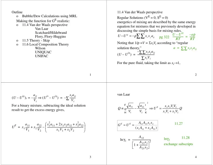
11.4 Van der Waals perspective Regular Solutions (VE = 0, SE = 0) energetics of mixing are described by the same energy equation for mixtures that we previously developed in discussing the simple basis for mixing rules. Noting that 1/ρ =V = ΣxiVi according to “regular solution theory,” For the pure fluid, taking the limit as xi→1, U U x x a

ig i j ij

− = −

∑ ∑

ρ U Uig – ( ) xixjaij

∑ ∑

– xiVi

∑

• =

pg 322 U Uig – RT

• aρ

– RT

• =

a xixjaij

∑ ∑

=

3

For a binary mixture, subtracting the ideal solution result to get the excess energy gives, U Uig – ( )i aii Vi

• –

= Uis Uig – ( ) ⇒ xiaii Vi

• ∑

– = UE x1 a11 V1

• x2

a22 V2

• x1

2a11

2x1x2a12 x2

2a22

+ + x1V1 x2V2 +

• 

     – + =

4

van Laar Q a V a V U x x V V x V x V Q

E

≡ −

F H G I K J

⇒ = +

11 1 22 2 2 1 2 1 2 1 1 2 2

G U A A x x x A x A

E E

= = +

12 21 1 2 1 12 2 21

( ) γ1 ln A12 1 A12x1 A21x2

• +

2

• =

11.27 lnγ2 exchange subscripts 11.28

SLIDE 2

5

Fitting Van Laar to a single experiment: Azeotrope point can be used. See example 11.6 A12 γ1 1 x2 γ2 ln x1 γ1 ln

• +

2

ln = A21 γ2 1 x1 γ1 ln x2 γ2 ln

• +

2

ln = yiP xiγiPi

sat

= γi yiP xiPi

sat

• P

Pi

sat

• =

=

6

Infinite dilution can be used. See example 11.7 ln γi γ1

∞

ln A12 = γ2

∞

ln x1

7

Scatchard Hildebrand a12= a a

11 22

UE x1x2V1V2 x1V1 x2V2 +

• a11

V1

2

• a22

V2

2

• 2 a11

V1

2

• a22

V2

2

• –

+       = UE x1x2V1V2 x1V1 x2V2 +

• a11

V1

• a22

V2

• –

     

2

= G U x V x V

E E

= = − + Φ Φ

1 2 1 2 2 1 1 2 2

δ δ

a f (

)

G U xV x V

E E

= = − + ΦΦ

1 2 1 2 2 1 1 2 2

δ δ

a f (

)

F i

i i i i

x V x V ∫

Â

/ is known as the "volume fraction"

8

This is a predictive technique valid for nonpolar

• substances. See table 11.1 for parameters.

Also can make adjustable. d i

ii i

a V ∫ / is known as the "solubility parameter" δ i

vap i vap i

U V H RT V ≡ − ∆ ∆ = a12 a1a2 1 k12 – ( ) = RT γ1 ln V1Φ2

2

δ1 δ2 – ( )2 2k12δ1δ2 + [ ] =

SLIDE 3

9

Van Laar and Scatchard-Hildbrand

330 335 340 345 350 355 0.2 0.4 0.6 0.8 1

x,y T(K)

Scatchard-Hildebrand kij=-0.038 van Laar

methanol + benzene MeOH

10

Flory’s Equation Recall Ideal Solution result (pg 95) S1 ∆ n1R VT V1

i

• ln

ntotx1R VT V1

i

• ln

= = S2 ∆ n2R VT V2

i

• ln

ntotx2R VT V2

i

• ln

= = n1 n2 permit mixing

11

S ∆ S1 ∆ S2 ∆ + ntotR x1 VT V1

i

• x2

VT V2

i

• ln

+ ln       = = free volume (not occupied) Vf i

,

niViλ = Vf n1V1 n2V2 + ( )λ =

12

G H TS RT x x x x

E E E

= − = + ( ln ln )

1 1 1 2 2 2

Φ Φ S ∆ nR x1 x1V1 x2V2 + ( )λ x1V1λ

• 

   ln x2 x1V1 x2V2 + ( )λ x2V2λ

• ln

+     = S

is

∆ nR x1 x1 ln x2 x2 ln + ( ) = SE S Sis – S xiSi

∑

– ( ) Sis xiSi

∑

– ( ) – S ∆ S ∆

is

– = = = athermal

SLIDE 4

13

Flory-Huggins Model GE RT x1 Φ1 x1

• ln

x2 Φ2 x2

• ln

+     Φ1Φ2 x1 x2R + ( )χRT + = Flory Scatchard-Hildebrand R V2 V1

• =

χ V1 δ1 δ2 – ( )2 RT

• =

χ = athermal However χ usually nonzero even with HE = 0 (compensate for error in Flory)

14

11.6 Local composition models (nonrandom) Common Features

• Lattice Model - Fixed number of neighbors = 10
• Uses GE = AE approximation (good)
• Local Composition

1 1 2 2 1 x21 - 2’s around 1 x11 - 1’s around 1 x12 - 1’s around 2 x22 - 2’s around 2

15

• Two-fluid Theory

x21 x11

• x2

x1

• Ω21

= x12 x22

• x1

x2

• Ω12

= U Uig – ( ) x1 U Uig – ( )

1 ( )

x2 U Uig – ( )

2 ( )

+ = UE NAz 2

• x1x2Ω21 ε21

ε11 – ( ) x1 x2Ω21 +

• x2x1Ω12 ε12

ε22 – ( ) x1Ω12 x2 +

• +

= AE RT

• UE

– RT

• T

d T

• ∫

C + =

16

Wilson’s equation Ω12 Λ21 V1 V2

• A

–

21

RT

• 

   exp = = γ1 ln x1 x2Λ12 + ( ) ln x2 Λ12 x1 x2Λ12 +

• Λ21

x1Λ21 x2 +

• –

    + – = integrate UE to get AE = GE (Eqn 11.85) differentiate GE to get γ expressions

SLIDE 5

17

UNIQUAC ri qi θi τij Ωij qi qj

• N

–

Az εij

εjj – ( ) 2RT

• 

   exp qi qj

• a

–

ij

T

• 

   exp qi qj

• τij

= = = q = surface area of molecule volume (look up) νkRk

groups

∑

surface area (look up) νkQk

groups

∑

xiqi ( ) xiqi

∑

( ) ⁄ surface area fractions a –

ij

T

• 

   exp = parameter

18

G RT x x x q x q x q x q x

E

= − + − + − +

1 1 1 2 2 1 1 1 1 2 2 2 2 1 1 1 2 21 2 2 1 12 2

ln / / ln / ln / ln( ) ln( ) Φ Φ Φ Φ

a f a f a f a f

+ x ln 5

2

θ θ θ θ τ θ τ θ

}

comb resid

}

Flory correction to Flory

19

γ1 ln Φ1 x1

• ln

1 Φ1 x1

• –

    5q1 Φ1 θ1

• ln

1 Φ1 θ1

• –

    + – q1 1 θ1 θ2τ21 + ( ) ln θ1 θ1 θ2τ21 +

• –

θ2τ12 θ1τ12 θ2 +

• –

– + + = γ2 ln Φ2 x2

• ln

1 Φ2 x2

• –

    5q2 Φ2 θ2

• ln

1 Φ2 θ2

• –

    + – q2 1 θ1τ12 θ2 + ( ) ln θ1τ21 θ1 θ2τ21 +

• –

θ2 θ1τ12 θ2 +

• –

– + + =

20

Group parameters for the UNIFAC and UNIQUAC equations. AC in the table means aromatic carbon. (DIFFERS SLIGHTLY FROM TEXT) Main Group Sub- group R(rel.vol.) Q(rel.area) Example CH2 CH3 0.9011 0.8480 CH2 0.6744 0.5400 n-hexane: 4 CH2+2 CH3 CH 0.4469 0.2280 isobutane: 1CH+3 CH3 C 0.2195 neopentane: 1C+ 4 CH3 C=C CH2=CH 1.2454 1.1760 1-hexene: 1 CH2=CH+3 CH2+1 CH3 CH=CH 1.1167 0.8670 2-hexene: 1 CH=CH+2 CH2+2 CH3 CH2=C 1.1173 0.9880 CH=C 0.8886 0.6760 C=C 0.6605 0.4850 ACH ACH 0.5313 0.4000 benzene: 6ACH AC 0.3652 0.1200 benzoic acid: 5ACH+1AC+1COOH ACCH2 ACCH3 1.2663 0.9680 toluene: 5ACH+1ACCH3 ACCH2 1.0396 0.6600 ethylbenzene: 5ACH+1ACCH2+1CH2 ACCH 0.8121 0.3480 OH OH 1.0000 1.2000 n-propanol: 1OH+1 CH3+2 CH2

SLIDE 6

21

CH3O H CH3OH 1.4311 1.4320 methanol is an independent group water H2O 0.9200 1.4000 water is an independent group furfural furfural 3.1680 2.4810 furfural is an independent group DOH (CH2OH) 2 2.4088 2.2480 ethylene glycol is an independent group ACOH ACOH 0.8952 0.6800 phenol: 1ACOH+5ACH CH2CO CH3CO 1.6724 1.4880 dimethylketone: 1 CH3CO+CH3 CH2CO 1.4457 1.1800 diethylketone=1 CH2CO+2 CH3+1 CH2 CHO CHO 0.9980 0.9480 acetaldehyde: 1CHO+1 CH3 CCOO CH2COO 1.9031 1.7280 methyl acetate: 1 CH3COO+1 CH3 CH2COO 1.6764 1.4200 methyl propanate: 1 CH2COO+2 CH3 COOH COOH 1.31013 1.2240 benzoic acid: 5ACH+1AC+1COOH Group parameters for the UNIFAC and UNIQUAC equations. AC in the table means aromatic carbon. (DIFFERS SLIGHTLY FROM TEXT)

22

UNIFAC

Pure 2-propanol CH3CHOHCH3 Hypothetical solution of “pure” CH3 Real mixture (SOG) CH3CHOHCH3 H2O CH3 H2O CH3CHOHCH3 H2O CH3CHOHCH3 CH3CHOHCH3 CH3 CH3 CH3

µCH3

SOG

µCH3

• –

µCH3

1 ( )

µCH3

• –

µCH3

SOG

µCH3

1 ( )

–

23

ln ln ln g g g

k k COMB k RES

= +

γ1

resid

ln µ1 µ1

• –

RT

• νm

1 ( )

Γm ln Γm

1 ( )

ln – [ ]

m

∑

= = γk

COMB

ln as UNIQUAC µCH3

SOG

µCH3

1 ( )

– RT

• µCH3

SOG

µCH3

• –

RT

• µCH3

1 ( )

µCH3

• –

RT

• –

ΓCH3 ln ΓCH3

1 ( )

ln – = = µ1 2µCH3

SOG

µCH

SOG

µOH

SOG

+ + = IPA µ1

• 2µCH3

1 ( )

µCH

1 ( )

µOH

1 ( )

+ + = mixture pure IPA

24 Group Variable Molecular Variable volume R r surface area Q q activity coefficient Γ γ surface fraction energy variable Ψij τij energy parameter aij aij mole fraction X x

Θ θ

SLIDE 7

25

compare to UNIQUAC eqns Γm ln Qm 1 ΘiΨim

i

∑

ln ΘjΨmj ΘiΨij

i

∑

• j

∑

– – = Θj surface area fraction of group j ( ) XjQj XiQi

i

∑

• ≡

= Ψmj a –

mj

T

• 

   exp = Xj νj

i ( )xi molecules i

∑

νk

i ( )xi groups k

∑

molecules i

∑

• =