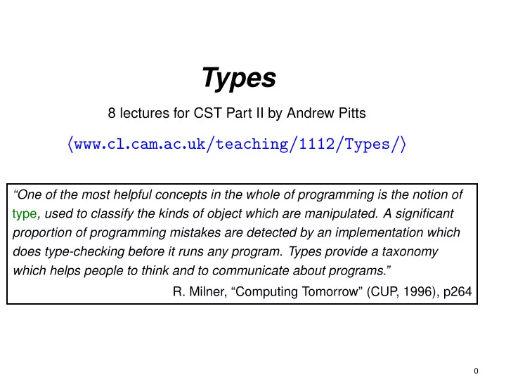
Types 8 lectures for CST Part II by Andrew Pitts www . cl . cam . - - PowerPoint PPT Presentation

Types

8 lectures for CST Part II by Andrew Pitts

www.cl.cam.ac.uk/teaching/1112/Types/

“One of the most helpful concepts in the whole of programming is the notion of type, used to classify the kinds of object which are manipulated. A significant proportion of programming mistakes are detected by an implementation which does type-checking before it runs any program. Types provide a taxonomy which helps people to think and to communicate about programs.”

• R. Milner, “Computing Tomorrow” (CUP

, 1996), p264

The full title of this course is

Type Systems for Programming Languages

What are ‘type systems’ and what are they good for? ‘A type system is a tractable syntactic method for proving the absence

• f certain program behaviours by classifying phrases according to the

kinds of values they compute’

• B. Pierce, ‘Types and Programming Languages’ (MIT, 2002), p1

Type systems are one of the most important channels by which developments in theoretical computer science get applied in programming language design and software verifiction.

1

Uses of type systems

• Detecting errors via type-checking, either statically (decidable errors

detected before programs are executed) or dynamically (typing errors detected during program execution).

• Abstraction and support for structuring large systems.
• Documentation.
• Efficiency.
• Whole-language safety.

2

Safety Informal definitions from the literature. ‘A safe language is one that protects its own high-level abstractions [no matter what legal program we write in it]’. ‘A safe language is completely defined by its programmer’s manual [rather than which compiler we are using]’. ‘A safe language may have trapped errors [one that can be handled gracefully], but can’t have untrapped errors [ones that cause unpredictable crashes]’.

3

Formal type systems

• Constitute the precise, mathematical characterisation of informal type

systems (such as occur in the manuals of most typed languages.)

• Basis for type soundness theorems: ‘any well-typed program cannot

produce run-time errors (of some specified kind)’.

• Can decouple specification of typing aspects of a language from

algorithmic concerns: the formal type system can define typing independently of particular implementations of type-checking algorithms.

4

Typical type system ‘judgement’ is a relation between typing environments (Γ), program phrases (M) and type expressions (τ ) that we write as

Γ ⊢ M : τ

and read as ‘given the assignment of types to free identifiers of M specified by type environment Γ, then M has type τ ’. E.g.

f : int list → int, b : bool ⊢ (if b then f nil else 3) : int

is a valid typing judgement about ML.

5

Notations for the typing relation ‘foo has type bar’ ML-style (used in this course):

foo : bar

Haskell-style:

foo :: bar

C/Java-style:

bar foo

6

Type checking, typeability, and type inference Suppose given a type system for a programming language with judgements of the form Γ ⊢ M : τ . Type-checking problem: given Γ, M, and τ , is Γ ⊢ M : τ derivable in the type system? Typeability problem: given Γ and M, is there any τ for which

Γ ⊢ M : τ is derivable in the type system?

Second problem is usually harder than the first. Solving it usually involves devising a type inference algorithm computing a τ for each Γ and M (or failing, if there is none).

7

Polymorphism = ‘has many types’ Overloading (or ‘ad hoc’ polymorphism): same symbol denotes

• perations with unrelated implementations. (E.g. + might mean both

integer addition and string concatenation.)

Subsumption τ1 <: τ2: any M1 : τ1 can be used as M1 : τ2 without violating safety. Parametric polymorphism (‘generics’): same expression belongs to a family of structurally related types. (E.g. in SML, length function

fun length nil = | length (x :: xs) = 1 + (length xs)

has type τ list → int for all types τ .)

8

Type variables and type schemes in Mini-ML To formalise statements like ‘ length has type τ list → int, for all types τ ’ it is natural to introduce type variables α (i.e. variables for which types may be substituted) and write

length : ∀ α (α list → int). ∀ α (α list → int) is an example of a type scheme.

9

Polymorphism of let-bound variables in ML For example in

let f = λx(x) in (f true) :: (f nil) λx(x) has type τ → τ for any type τ , and the variable f to which it is

bound is used polymorphically:

• in (f true), f has type bool → bool
• in (f nil), f has type bool list → bool list

Overall, the expression has type bool list.

10

‘Ad hoc’ polymorphism: if f : bool → bool and f : bool list → bool list, then (f true) :: (f nil) : bool list. ‘Parametric’ polymorphism: if f : ∀ α (α → α), then (f true) :: (f nil) : bool list.

11

Mini-ML types and type schemes Types

τ ::= α

type variable

| bool

type of booleans

| τ → τ

function type

| τ list

list type where α ranges over a fixed, countably infinite set TyVar. Type Schemes

σ ::= ∀ A (τ)

where A ranges over finite subsets of the set TyVar. When A = {α1, . . . , αn}, we write ∀ A (τ) as

∀ α1, . . . , αn (τ).

12

The ‘generalises’ relation between type schemes and types We say a type scheme σ = ∀ α1, . . . , αn (τ ′) generalises a type

τ , and write σ ≻ τ

if τ can be obtained from the type τ ′ by simultaneously substituting some types τi for the type variables αi (i = 1, . . . , n):

τ = τ ′[τ1/α1, . . . , τn/αn].

(N.B. The relation is unaffected by the particular choice of names of bound type variables in σ.)

The converse relation is called specialisation: a type τ is a specialisation

• f a type scheme σ if σ ≻ τ .

13

Mini-ML typing judgement takes the form Γ ⊢ M : τ where

• the typing environment Γ is a finite function from variables to type

schemes. (We write Γ = {x1 : σ1, . . . , xn : σn} to indicate that Γ has domain of definition dom(Γ) = {x1, . . . , xn} and maps each

xi to the type scheme σi for i = 1..n.)

• M is an Mini-ML expression
• τ is an Mini-ML type.

14

Mini-ML expressions, M

::= x

variable

| true

boolean values

| false | if M then M else M

conditional

| λx(M)

function abstraction

| M M

function application

| let x = M in M

local declaration

| nil

nil list

| M :: M

list cons

| case M of nil = > M | x :: x = > M

case expression

15

Mini-ML type system, I

Γ ⊢ x : τ

if (x : σ) ∈ Γ and σ ≻ τ (var ≻)

Γ ⊢ B : bool

if B ∈ {true, false} (bool)

Γ ⊢ M1 : bool Γ ⊢ M2 : τ Γ ⊢ M3 : τ Γ ⊢ if M1 then M2 else M3 : τ

(if)

16

Mini-ML type system, II

Γ ⊢ nil : τ list

(nil)

Γ ⊢ M1 : τ Γ ⊢ M2 : τ list Γ ⊢ M1 :: M2 : τ list

(cons)

Γ ⊢ M1 : τ1 list Γ ⊢ M2 : τ2 Γ, x1 : τ1, x2 : τ1 list ⊢ M3 : τ2 Γ ⊢ case M1 of nil = > M2 |x1 :: x2 = > M3 : τ2

if x1, x2 /

∈ dom(Γ)

and x1 = x2 (case)

17

Mini-ML type system, III

Γ, x : τ1 ⊢ M : τ2 Γ ⊢ λx(M) : τ1 → τ2

if x /

∈ dom(Γ)

(fn)

Γ ⊢ M1 : τ1 → τ2 Γ ⊢ M2 : τ1 Γ ⊢ M1 M2 : τ2

(app)

18

Mini-ML type system, IV

Γ ⊢ M1 : τ Γ, x : ∀ A (τ) ⊢ M2 : τ ′ Γ ⊢ let x = M1 in M2 : τ ′

if x /

∈ dom(Γ) and A = ftv(τ) − ftv(Γ)

(let)

19

Assigning type schemes to Mini-ML expressions Given a type scheme σ = ∀ A (τ), write

Γ ⊢ M : σ

if A = ftv(τ) − ftv(Γ) and Γ ⊢ M : τ is derivable from the axiom and rules on Slides 16–19. When Γ = { } we just write

⊢ M : σ for { } ⊢ M : σ and say

that the (necessarily closed—see Exercise 2.5.2) expression M is typeable in Mini-ML with type scheme σ.

20

Two examples involving self-application

M

def

= let f = λx1(λx2(x1)) in f f M ′ def = (λf(f f)) λx1(λx2(x1))

Are M and M ′ typeable in the Mini-ML type system?

21

Constraints generated while inferring a type for

let f = λx1(λx2(x1)) in f f A = ftv(τ2)

(C0)

τ2 = τ3 → τ4

(C1)

τ4 = τ5 → τ6

(C2)

∀ { } (τ3) ≻ τ6, i.e. τ3 = τ6

(C3)

τ7 = τ8 → τ1

(C4)

∀ A (τ2) ≻ τ7

(C5)

∀ A (τ2) ≻ τ8

(C6)

22

Principal type schemes for closed expressions A closed type scheme ∀ A (τ) is the principal type scheme of a closed Mini-ML expression M if (a) ⊢ M : ∀ A (τ) (b) for any other closed type scheme ∀ A′ (τ ′), if ⊢ M : ∀ A′ (τ ′), then ∀ A (τ) ≻ τ ′

23

Theorem (Hindley; Damas-Milner) If the closed Mini-ML expression M is typeable (i.e. ⊢ M : σ holds for some type scheme σ), then there is a principal type scheme for M. Indeed, there is an algorithm which, given any M as input, decides whether or not it is typeable and returns a principal type scheme if it is.

24

An ML expression with a principal type scheme hundreds of pages long

let pair = λx(λy(λz(z x y))) in let x1 = λy(pair y y) in let x2 = λy(x1(x1 y)) in let x3 = λy(x2(x2 y)) in let x4 = λy(x3(x3 y)) in let x5 = λy(x4(x4 y)) in x5(λy(y))

(Taken from Mairson 1990.)

25

Unification of ML types There is an algorithm mgu which when input two Mini-ML types τ1 and

τ2 decides whether τ1 and τ2 are unifiable, i.e. whether there exists a

type-substitution S ∈ Sub with (a) S(τ1) = S(τ2). Moreover, if they are unifiable, mgu(τ1, τ2) returns the most general unifier—an S satisfying both (a) and (b) for all S′ ∈ Sub, if S′(τ1) = S′(τ2), then S′ = T S for some

T ∈ Sub.

By convention mgu(τ1, τ2) = FAIL if (and only if) τ1 and τ2 are not unifiable.

26

Principal type schemes for open expressions A solution for the typing problem Γ ⊢ M : ? is a pair (S, σ) consisting of a type substitution S and a type scheme σ satisfying

S Γ ⊢ M : σ

(where S Γ = {x1 : S σ1, . . . , xn : S σn}, if

Γ = {x1 : σ1, . . . , xn : σn}).

Such a solution is principal if given any other, (S′, σ′), there is some

T ∈ Sub with T S = S′ and T (σ) ≻ σ′.

[For type schemes σ and σ′, with σ′ = ∀ A′ (τ ′) say, we define

σ ≻ σ′ to mean A′ ∩ ftv(σ) = {} and σ ≻ τ ′.]

27

Properties of the Mini-ML typing relation

• If Γ ⊢ M : σ, then for any type substitution S ∈ Sub

SΓ ⊢ M : Sσ.

• If Γ ⊢ M : σ and σ ≻ σ′, then Γ ⊢ M : σ′.

28

Specification for the principal typing algorithm, pt

pt operates on typing problems Γ ⊢ M : ? (consisting of a typing

environment Γ and a Mini-ML expression M). It returns either a pair

(S, τ) consisting of a type substitution S ∈ Sub and a Mini-ML type τ , or the exception FAIL.

• If Γ ⊢ M : ? has a solution (cf. Slide 27), then pt(Γ ⊢ M : ?)

returns (S, τ) for some S and τ ; moreover, setting A = (ftv(τ) − ftv(S Γ)), then

(S, ∀ A (τ)) is a principal solution for the problem Γ ⊢ M : ?.

• If Γ ⊢ M : ? has no solution, then pt(Γ ⊢ M : ?) returns

FAIL.

29

Some of the clauses in a definition of pt Function abstractions: pt(Γ ⊢ λx(M) : ?)

def

= let α = fresh in let (S, τ) = pt(Γ, x : α ⊢ M : ?) in (S, S(α) → τ)

Function applications: pt(Γ ⊢ M1 M2 : ?)

def

= let (S1, τ1) = pt(Γ ⊢ M1 : ?) in let (S2, τ2) = pt(S1 Γ ⊢ M2 : ?) in let α = fresh in let S3 = mgu(S2 τ1, τ2 → α) in (S3S2S1, S3(α))

30

ML types and expressions for mutable references

τ ::= . . . | unit

unit type

| τ ref

reference type.

M ::= . . . | ()

unit value

| ref M

reference creation

| !M

dereference

| M := M

assignment

31

Midi-ML’s extra typing rules

Γ ⊢ () : unit

(unit)

Γ ⊢ M : τ Γ ⊢ ref M : τ ref

(ref)

Γ ⊢ M : τ ref Γ ⊢ !M : τ

(get)

Γ ⊢ M1 : τ ref Γ ⊢ M2 : τ Γ ⊢ M1 := M2 : unit

(set)

32

Example 3.1.1 The expression

let r = ref λx(x) in let u = (r := λx′(ref !x′)) in (!r)()

has type unit.

33

Midi-ML transitions involving references

!x, s → s(x), s

if x ∈ dom(s)

!V, s → FAIL

if V not a variable

x := V ′, s → (), s[x → V ′] V := V ′, s → FAIL

if V not a variable

ref V, s → x, s[x → V ]

if x /

∈ dom(s)

where V ranges over values:

V ::= x | λx(M) | () | true | false | nil | V :: V

34

Value-restricted typing rule for let-expressions

Γ ⊢ M1 : τ1 Γ, x : ∀ A (τ1) ⊢ M2 : τ2 Γ ⊢ let x = M1 in M2 : τ2 (†)

(letv)

(†) provided x / ∈ dom(Γ) and A =

• { }

if M1 is not a value

ftv(τ1) − ftv(Γ)

if M1 is a value

(Recall that values are given by

V ::= x | λx(M) | () | true | false | nil | V :: V .)

35

Type soundness for Midi-ML with the value restriction For any closed Midi-ML expression M, if there is some type scheme σ for which

⊢ M : σ

is provable in the value-restricted type system (axioms and rules on Slides 16–18, 32 and 35), then evaluation of M does not fail, i.e. there is no sequence of transitions of the form

M, { } → · · · → FAIL

for the transition system → defined in Figure 4 (where { } denotes the empty state).

36

λ-bound variables in ML cannot be used

polymorphically within a function abstraction

E.g. λf((f true) :: (f nil)) and λf(f f) are not typeable in the ML type system.

Syntactically, because in rule

(fn) Γ, x : τ1 ⊢ M : τ2 Γ ⊢ λx(M) : τ1 → τ2

the abstracted variable has to be assigned a trivial type scheme (recall

x : τ1 stands for x : ∀ { } (τ1)).

Semantically, because ∀ A (τ1) → τ2 is not semantically equivalent to an ML type when A = { }.

37

Monomorphic types . . .

τ ::= α | bool | τ → τ | τ list

. . . and type schemes

σ ::= τ | ∀ α (σ)

Polymorphic types

π ::= α | bool | π → π | π list | ∀ α (π)

E.g. α → α′ is a type, ∀ α (α → α′) is a type scheme and a polymorphic type (but not a monomorphic type), ∀ α (α) → α′ is a polymorphic type, but not a type scheme.

38

Identity, Generalisation and Specialisation

Γ ⊢ x : π

if (x : π) ∈ Γ (id)

Γ ⊢ M : π Γ ⊢ M : ∀ α (π)

if α /

∈ ftv(Γ)

(gen)

Γ ⊢ M : ∀ α (π) Γ ⊢ M : π[π′/α]

(spec)

39

Fact (see Wells 1994): For the modified ML type system with polymorphic types and (var ≻) replaced by the axiom and rules on Slide 39, the type checking and typeability problems (cf. Slide 7) are equivalent and undecidable.

40

Explicitly versus implicitly typed languages Implicit: little or no type information is included in program phrases and typings have to be inferred (ideally, entirely at compile-time). (E.g. Standard ML.) Explicit: most, if not all, types for phrases are explicitly part of the syntax. (E.g. Java.)

E.g. self application function of type ∀ α (α) → ∀ α (α) (cf. Example 4.1.1) Implicitly typed version: λ f (f f) Explicitly type version: λ f : ∀ α1 (α1) (Λ α2 (f(α2 → α2)(f α2)))

41

PLC syntax Types

τ ::= α

type variable

| τ → τ

function type

| ∀ α (τ) ∀-type

Expressions

M ::= x

variable

| λ x : τ (M)

function abstraction

| M M

function application

| Λ α (M)

type generalisation

| M τ

type specialisation

(α and x range over fixed, countably infinite sets TyVar and Var respectively.)

42

Functions on types In PLC, Λ α (M) is an anonymous notation for the function F mapping each type τ to the value of M[τ/α] (of some particular type).

F τ

denotes the result of applying such a function to a type. Computation in PLC involves beta-reduction for such functions on types

(Λ α (M)) τ → M[τ/α]

as well as the usual form of beta-reduction from λ-calculus

(λ x : τ (M1)) M2 → M1[M2/x]

43

PLC typing judgement takes the form Γ ⊢ M : τ where

• the typing environment Γ is a finite function from variables to PLC

types. (We write Γ = {x1 : τ1, . . . , xn : τn} to indicate that Γ has domain of definition dom(Γ) = {x1, . . . , xn} and maps each

xi to the PLC type τi for i = 1..n.)

• M is a PLC expression
• τ is a PLC type.

44

PLC type system

Γ ⊢ x : τ

if (x : τ) ∈ Γ (var)

Γ, x : τ1 ⊢ M : τ2 Γ ⊢ λ x : τ1 (M) : τ1 → τ2

if x /

∈ dom(Γ)

(fn)

Γ ⊢ M1 : τ1 → τ2 Γ ⊢ M2 : τ1 Γ ⊢ M1 M2 : τ2

(app)

Γ ⊢ M : τ Γ ⊢ Λ α (M) : ∀ α (τ)

if α /

∈ ftv(Γ)

(gen)

Γ ⊢ M : ∀ α (τ1) Γ ⊢ M τ2 : τ1[τ2/α]

(spec)

45

An incorrect ‘proof’

x1 : α, x2 : α ⊢ x2 : α (var) x1 : α ⊢ λ x2 : α (x2) : α → α (fn) x1 : α ⊢ Λ α (λ x2 : α (x2)) : ∀ α (α → α) (wrong!)

46

Decidability of the PLC typeability and type-checking problems Theorem. For each PLC typing problem, Γ ⊢ M : ?, there is at most one PLC type τ for which Γ ⊢ M : τ is provable. Moreover there is an algorithm, typ, which when given any Γ ⊢ M : ? as input, returns such a τ if it exists and FAILs otherwise. Corollary. The PLC type checking problem is decidable: we can decide whether or not Γ ⊢ M : τ is provable by checking whether

typ(Γ ⊢ M : ?) = τ .

(N.B. equality of PLC types up to alpha-conversion is decidable.)

47

PLC type-checking algorithm, I Variables:

typ(Γ, x : τ ⊢ x : ?)

def

= τ

Function abstractions:

typ(Γ ⊢ λ x : τ1 (M) : ?)

def

= let τ2 = typ(Γ, x : τ1 ⊢ M : ?) in τ1 → τ2

Function applications:

typ(Γ ⊢ M1 M2 : ?)

def

= let τ1 = typ(Γ ⊢ M1 : ?) in let τ2 = typ(Γ ⊢ M2 : ?) in case τ1 of τ → τ ′ → if τ = τ2 then τ ′ else FAIL | → FAIL

48

PLC type-checking algorithm, II Type generalisations:

typ(Γ ⊢ Λ α (M) : ?)

def

= let τ = typ(Γ ⊢ M : ?) in ∀ α (τ)

Type specialisations:

typ(Γ ⊢ M τ2 : ?)

def

= let τ = typ(Γ ⊢ M : ?) in case τ of ∀ α (τ1) → τ1[τ2/α] | → FAIL

49

Beta-reduction of PLC expressions

M beta-reduces to M ′ in one step, M → M ′ , means M ′ can be obtained from M (up to alpha-conversion, of course) by

replacing a subexpression which is a redex by its corresponding reduct. The redex-reduct pairs are of two forms:

(λ x : τ (M1)) M2 → M1[M2/x] (Λ α (M)) τ → M[τ/α]. M →∗ M ′ indicates a chain of finitely† many beta-reductions.

(† possibly zero—which just means M and M ′ are alpha-convertible).

M is in beta-normal form if it contains no redexes.

50

Properties of PLC beta-reduction on typeable expressions Suppose Γ ⊢ M : τ is provable in the PLC type system. Then the following properties hold: Subject Reduction. If M → M ′, then Γ ⊢ M ′ : τ is also a provable typing. Church Rosser Property. If M →∗ M1 and M →∗ M2, then there is M ′ with M1 →∗ M ′ and M2 →∗ M ′. Strong Normalisation Property. There is no infinite chain

M → M1 → M2 → . . . of beta-reductions starting from M.

51

PLC beta-conversion, =β By definition, M =β M ′ holds if there is a finite chain

M − · − · · · − · − M ′

where each − is either → or ←, i.e. a beta-reduction in one direction or the other. (A chain of length zero is allowed—in which case M and M ′ are equal, up to alpha-conversion, of course.) Church Rosser + Strong Normalisation properties imply that, for typeable PLC expressions, M =β M ′ holds if and only if there is some beta-normal form N with

M →∗ N ∗← M ′

52

Polymorphic booleans

bool

def

= ∀ α (α → (α → α)) True

def

= Λ α (λ x1 : α, x2 : α (x1)) False

def

= Λ α (λ x1 : α, x2 : α (x2)) if

def

= Λ α (λ b : bool, x1 : α, x2 : α (b α x1 x2))

53

Polymorphic lists

α list

def

= ∀ α′ (α′ → (α → α′ → α′) → α′) Nil

def

= Λ α, α′ (λ x′ : α′, f : α → α′ → α′ (x′)) Cons

def

= Λα(λx : α, ℓ : α list(Λα′( λx′ : α′, f : α → α′ → α′( f x (ℓ α′ x′ f)))))

54

Iteratively defined functions on finite lists

A∗ def = finite lists of elements of the set A

Given a set A′, an element x′ ∈ A′, and a function

f : A → A′ → A′, the iteratively defined function listIter x′ f is

the unique function g : A∗ → A′ satisfying:

g Nil = x′ g (x :: ℓ) = f x (g ℓ).

for all x ∈ A and ℓ ∈ A∗.

55

List iteration in PLC

iter

def

= Λα, α′(λx′ : α′, f : α → α′ → α′( λ ℓ : α list (ℓ α′ x′ f)))

satisfies:

• ⊢ iter : ∀ α, α′ (α′ → (α → α′ → α′) → α list → α′)
• iter α α′ x′ f (Nil α) =β x′
• iter α α′ x′ f (Cons α x ℓ) =β f x (iter α α′ x′ f ℓ)

56

A tautology checker

fun taut n f = if n = 0 then f else (taut(n − 1)(f true)) andalso (taut(n − 1)(f false))

Defining types

• 0 AryBoolOp

def

= bool (n + 1) AryBoolOp

def

= bool → (n AryBoolOp)

then taut n has type (n AryBoolOp) → bool, i.e. the result type

• f the function taut depends upon the value of its argument.

57

The tautology checker in Agda

data Bool : Set where True : Bool False : Bool _and_ : Bool -> Bool -> Bool True and True = True True and False = False False and _ = False data Nat : Set where Zero : Nat Succ : Nat -> Nat

_AryBoolOp : Nat -> Set Zero AryBoolOp = Bool (Succ n) AryBoolOp = Bool -> n AryBoolOp taut : (n : Nat) -> n AryBoolOp -> Bool taut Zero f = f taut (Succ n) f = taut n (f True) and taut n (f False)

58

Dependent function types (x : τ) → τ ′

Γ, x : τ ⊢ M : τ ′ Γ ⊢ λ x : τ (M) : (x : τ) → τ ′

if x /

∈ dom(Γ) ∪ fv(Γ) Γ ⊢ M : (x : τ) → τ ′ Γ ⊢ M ′ : τ Γ ⊢ M M ′ : τ ′[M ′/x] τ ′ may ‘depend’ on x, i.e. have free occurrences of x.

(Free occurrences of x in τ ′ are bound in (x : τ) → τ ′.)

59

Curry-Howard correspondence Logic

↔

Type system propositions, φ

↔

types, τ (constructive) proofs, p

↔

expressions, M ‘p is a proof of φ’

↔

‘M is an expression of type τ ’ simplification of proofs

↔

reduction of expressions

60

Second-order intuitionistic propositional calculus (2IPC) 2IPC propositions: φ ::= p | φ → φ | ∀ p (φ) , where p ranges

• ver an infinite set of propositional variables.

2IPC sequents: Φ ⊢ φ , where Φ is a finite set of 2IPC propositions and φ is a 2IPC proposition.

Φ ⊢ φ is provable if it is in the set of sequents inductively generated by:

(Id) Φ ⊢ φ if φ ∈ Φ (→I)

Φ, φ ⊢ φ′ Φ ⊢ φ → φ′

(→E) Φ ⊢ φ → φ′

Φ ⊢ φ Φ ⊢ φ′

(∀I)

Φ ⊢ φ Φ ⊢ ∀ p (φ)

if p /

∈ fv(Φ)

(∀E)

Φ ⊢ ∀ p (φ) Φ ⊢ φ[φ′/p]

61

A 2IPC proof {p & q, p, q} ⊢ p (Id) {p & q, p} ⊢ q → p (→I) {p & q} ⊢ p → q → p (→I) {p & q} ⊢ ∀ r ((p → q → r) → r) (Id) {p & q} ⊢ (p → q → p) → p (∀E) {p & q} ⊢ p (→E) { } ⊢ p & q → p (→I) { } ⊢ ∀ q (p & q → p) (∀I) { } ⊢ ∀ p, q (p & q → p) (∀I) where p & q is an abbreviation for ∀ r ((p → q → r) → r). The PLC expression corresponding to this proof is:

Λ p, q (λ z : p & q (z p (λ x : p, y : q (x)))).

62

Type-inference versus proof search Type-inference: ‘given Γ and M, is there a type σ such that

Γ ⊢ M : σ?’

(For PLC/2IPC this is decidable.) Proof-search: ‘given Γ and σ, is there a proof term M such that

Γ ⊢ M : σ?’

(For PLC/2IPC this is undecidable.)

63

2IPC is a constructive logic For example, there is no proof of the Law of Excluded Middle

∀ p (p ∨ ¬p)

Using the definitions on Slide 65, this is an abbreviation for

∀ p, q ((p → q) → ((p → ∀ r (r)) → q) → q)

(The fact that there is no closed PLC term of type ∀ p (p ∨ ¬p) can be proved using the technique developed in the Tripos question 13 on paper 9 in 2000.)

64

Logical operations definable in 2IPC

• Truth: true

def

= ∀ p (p → p).

• Falsity: false

def

= ∀ p (p).

• Conjunction: φ & φ′ def

= ∀ p ((φ → φ′ → p) → p)

(where p /

∈ fv(φ, φ′)).

• Disjunction: φ ∨ φ′ def

= ∀ p ((φ → p) → (φ′ → p) → p)

(where p /

∈ fv(φ, φ′)).

• Negation: ¬φ

def

= φ → false.

• Existential quantification:

∃ p (φ)

def

= ∀ p′ (∀ p (φ → p′) → p′)

(where p′ /

∈ fv(φ, p)).

65

Example of a non-constructive proof

• Theorem. There exist two irrational numbers a and b such that ba is

rational.

• Proof. Either √2

√2 is rational, or it is not (LEM!).

If it is, we can take a = b = √2, since √2 is irrational by a well-known theorem attributed to Euclid. If it is not, we can take a = √2 and b = √2

√2, since then

ba = (√2

√2) √2 = √2 √2×√2 = √22 = 2.

QED

66