Transition Path Theory TPT: method to study the ensemble of reactive - PowerPoint PPT Presentation

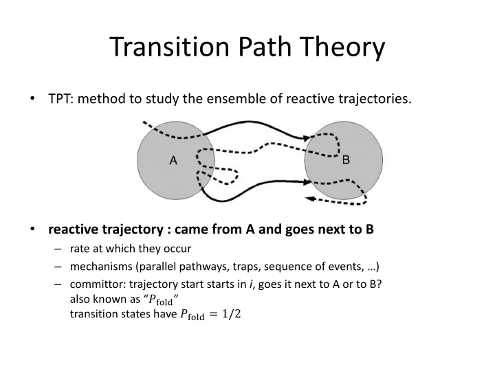
Transition Path Theory TPT: method to study the ensemble of reactive trajectories. • reactive trajectory : came from A and goes next to B • – rate at which they occur – mechanisms (parallel pathways, traps, sequence of events, …) – committor: trajectory start starts in i , goes it next to A or to B? also known as “ ! "#$% ” transition states have ! "#$% = 1/2

The committor A drunk man walks one block left with P=1/2 and one block right • with P=1/2. Probability that the man starting in block i will reach home before • the bar? 0 i-1 i i+1 N !(#) = 0 N=bar. No chance to reach home if already at bar. • !(0) = 1 0=home. If at home, 100% chance to reach home. • !(() for ∉ {0, #} ? • Doyle, Snell , Random Walks and Electric Networks , Carus (1984) Image: Valleriani, Nat. Scientific Reports 5, 17986 (2015).

# The committor ! " $(0) = 1 , $ * = 0 , $(+) for ∉ {0, *} ? 0 i-1 i i+1 N Start with general statement from probability theory: E event, F and G event s. t. only one of G or F will occur $(0) = $(0|2) $(2) + $(0|4) $(4) E = the man reaches home first F = the first step is to the right G = the first step is to the left P(home)= P(home| went right) P(went right) + P(home | went left) P(went left) P(home from i )= P(home from i +1) P(went right) + P(home from i -1) P(went left) # = ! "#5 # 6 ","#5 + ! "75 # 6 ","75 ! "

# The committor ! " The same argument that we made for a 1-D random walk can be make for a general kinetic network (MSM). The equations from the last slides are generalized to: # = 0 for & ∈ ( ! " • # = 1 for & ∈ * ! " • # = ∑ ,∈- . ", ! , # for & ∉ {(, *} ! " • 0 < ! # < 1 ! # = 1 ! # = 0 3 that gives the probability of (immediately) There exists also a committor ! " coming from a set A without having visited B in between. For reversible systems 3 = 1 − ! " # ! "

Reactive probability flux ! "# Reactive flux : average number of reactive trajectories per time unit making a transition from i to j on their way from A to B . Misnomer, really should be “current”, unit = 1/time unit . if / ≠ 1 + , % - %& * & "# : = )* % $ %& 0 if / = 1 i j Properties (essentially the properties of electric current): Flux conservation within the intermediate states (Kirchhoff’s law) • "# − $ "# ) = 0 for all / ∉ {A, B} ∑ & ($ %& &% What goes into the network in A comes out at B: • "# = "# ? $ ? $ %& %& %∈",&∉" %∉#,&∈#

Example transition probabilities:

Example reactive gross flux: 0.0031 + 0.0077 = 0.0108 = 0.0036 + 0.0072

Gross flux vs. Net flux On their way from A to B , trajectories might take forward and backward steps. What if we were only interested in the productive flux, that is in steps that take us closer to B ? Define the net flux : $ = max ! )* − ! )* , 0 ! "# "# #" for reversible systems one can show that $ = max . " / "# 0 # $ − 0 " $ , 0 ! "#

Example reactive gross flux:

Example reactive net flux:

Pathway decomposition A pathway is a sequence of states that starts with a state in A and ends • with a state in B ! = ($ % , $ ' , … , $ ) ) such that $ % ∈ , , $ ) ∈ - You can think of a pathway a special network without meshes (loops). • There is also a flux matrix . / for the pathway. We aim to decompose the network into a number of pathways. • The original network should be the “sum” of all the pathways. • . 0 = 1 . 2345 ) ) The pathway decomposition of the network will use an algorithm that • “subtracts” pathways from the original network.

Example

Example

Example

Example

Example

Example

Further reading • F. Noé, C. Schütte, E. Vanden-Eijnden, L. Reich, T. Weikl: “Constructing the Full Ensemble of Folding Pathways from Short Off-Equilibrium Simulations”. • P. Metzner, C. Schütte, and E. Vanden-Eijnden: “Transition Path Theory for Markov Jump Processes”. Mult. Mod. Sim. (2007)

• The capacity (or flux) of pathway is its weakest link ! " = min{! ( ) ( )*+ ∣ - = 1 … 0 − 1} • Pathway decomposition: chose a pathway " 3 and remove its capacity from the flux along all edges of " 3 . Repeat until no flux remains.

outline • Committor • Reactive flux • Gross flux vs. Net flux • Pathway decomposition • A word of caution

Gross flux vs. Net flux On their way from A to B , trajectories might take forward and backward steps. What if we were only interested in the productive flux, that is in steps that take us closer to B ? $ = max ! )* − ! )* , 0 Define the net flux : ! "# "# #" for the case of detailed balance one can show that $ = max . " / "# 0 # $ − 0 " $ , 0 ! "# $ might still contain (For the general case, without detailed balance ! "# unproductive cycles/detours.)

Transition Path Theory Computer tutorial in Markov modeling (PyEMMA) 20.2.2018 Fabian Paul

Coarse-graining of fluxes Markov model construction is best done with many states. For better interpretation you may be interested in a coarse-grained version of the state space (e.g. PCCA sets / metastable sets). Reactive currents are a quantity that can be coarse-grained without systematic error. (In contrast a to coarse-grained transition matrix). $% = ∑ (∈",+∈# , $% where - ∩ (0 ∪ 2) = ∅ and 5 ∩ (0 ∪ 2) = ∅ ! "# (+ + +

The committor # is defined as the probability that The discrete forward committor ! " the process starting in i will reach first B (home) rather than A (bar). # = ! "#% # & ","#% + ! ")% # & ",")% ! " Same argument works for general MSM and a “home“ and “bar“ that consists of more than of one MSM state. # = 0 for + ∈ - ! " • # = 1 for + ∈ / ! " • # = ∑ 1∈2 & "1 ! 1 # for + ∉ {-, /} ! " • For the reverse process ) = 1 for + ∈ - ! " • ) = 0 for + ∈ / ! " • 0 < ! # < 1 ! # = 1 ) = ∑ 1∈2 ) for + ∉ {-, /} ! # = 0 67 ! " 68 & 1" ! 1 • ) = 1 − ! " # With detailed balance ! "

Pathway decomposition • pathway ! = ($ % , $ ' , … , $ ) ) such that $ % ∈ , , $ ) ∈ - • capacity (or flux) of pathway . ! = min{. 3 4 3 456 ∣ 8 = 1 … : − 1} • Pathway decomposition: chose a pathway ! % and remove its capacity from the flux along all edges of ! % . Repeat until no flux remains. • Decomposition is not unique, depends on the order in which ! % , ! ' , … are picked. Reasonable choice: remove the strongest pathway (the one with largest capacity) first, then remove the strongest pathway of the remaining network.