
SLIDE 1
Trajectory Clustering: Visual Analytics Approaches Gennady Andrienko - - PowerPoint PPT Presentation
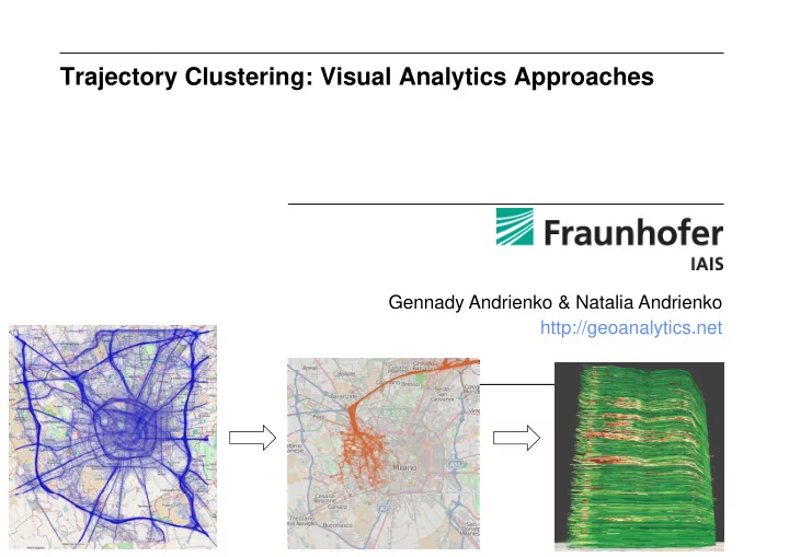
Trajectory Clustering: Visual Analytics Approaches Gennady Andrienko & Natalia Andrienko y http://geoanalytics.net Outline Similarity measures for trajectories Si il it f t j t i Density-based clustering of trajectories
2 http://geoanalytics.net
3
http://geoanalytics.net
4
http://geoanalytics.net
Travelled distance
5
http://geoanalytics.net
6
http://geoanalytics.net
7 http://geoanalytics.net
8
http://geoanalytics.net
9
Cluster 1 Cluster 2
http://geoanalytics.net
10 http://geoanalytics.net
11 http://geoanalytics.net
12 http://geoanalytics.net
13 http://geoanalytics.net
14 http://geoanalytics.net
15 http://geoanalytics.net
16 http://geoanalytics.net
17 http://geoanalytics.net
18 http://geoanalytics.net
19 http://geoanalytics.net
20 http://geoanalytics.net
21 http://geoanalytics.net
22 http://geoanalytics.net
23 http://geoanalytics.net
24 http://geoanalytics.net
25
http://geoanalytics.net
26 http://geoanalytics.net
27 http://geoanalytics.net
28
http://geoanalytics.net
29 http://geoanalytics.net
30
http://geoanalytics.net
31
http://geoanalytics.net
32 http://geoanalytics.net
33 http://geoanalytics.net
34
http://geoanalytics.net
35
http://geoanalytics.net
36 http://geoanalytics.net
37 http://geoanalytics.net
38 http://geoanalytics.net
39 http://geoanalytics.net
40 http://geoanalytics.net
41 http://geoanalytics.net
42 http://geoanalytics.net
43 http://geoanalytics.net
Round Number of clusters found in the subset Maximum cluster size in the subset Maximum cluster size in the database 1 28 37 87 74 1525 2 23 22 488
3 17 27 418 4 18 16 289
44
http://geoanalytics.net
45
http://geoanalytics.net
46 http://geoanalytics.net
47 http://geoanalytics.net
48
http://geoanalytics.net
49 http://geoanalytics.net
50 http://geoanalytics.net
51 http://geoanalytics.net
52 http://geoanalytics.net
53 http://geoanalytics.net
54
http://geoanalytics.net