SLIDE 1
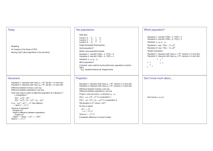
Today.
Modelling. An Analysis of the Power of PCA. Musing (rant?) about algorithms in the real world.
Two populations.
DNA data: human1: A ··· C ··· T ··· A human2: C ··· C ··· A ··· T human3: A ··· G ··· T ··· T Single Nucleotide Polymorphism. Same population? Model: same populution breeds. Population 1: snp 843: Pr[A] = .4 , Pr[T] = .6 Population 2: snp 843: Pr[A] = .6 , Pr[T] = .4 Individual: x1,x2,x3..,xn. Which population? Comment: snps could be movie preferences, populations could be types. E.g., republican/democrat, shopper/saver.
Which population?
Population 1: snp 843: Pr[A] = .4 , Pr[T] = .6 Population 2: snp 843: Pr[A] = .6 , Pr[T] = .4 Individual: x1,x2,x3..,xn. Population 1: snp i: Pr[xi = 1] = p(1)
i
Population 2: snp i: Pr[xi = 1] = p(2)
i
Simpler Calculation: Population 1: Gaussion with mean µ1 ∈ Rd, variance σ in each dim. Population 2: Gaussion with mean µ2 ∈ Rd, variance σ in each dim.
Gaussians
Population 1: Gaussion with mean µ1 ∈ Rd, std dev. σ in each dim. Population 2: Gaussion with mean µ2 ∈ Rd, std dev. σ in each dim. Difference between humans σ per snp. Difference between populations ε per snp. How many snps to collect to determine population for individual x? x in population 1. E[(x − µ1)2] = dσ2 E[(x − µ2)2] ≥ (d −1)σ2 +(µ1 − µ2)2. If (µ1 − µ2)2 = dε2 >> σ2, then different. → take d >> σ2/ε2 Variance of estimator? Roughly dσ4. Signal is difference between expecations. roughly dε2 Signal >> Noise. ↔ dε2 >> √ dσ2. Need d >> σ4/ε4.
Projection
Population 1: Gaussion with mean µ1 ∈ Rd, variance σ in each dim. Population 2: Gaussion with mean µ2 ∈ Rd, variance σ in each dim. Difference between humans σ per snp. Difference between populations ε per snp. Project x onto unit vector v in direction µ2 − µ1. E[((x − µ1)·v)2] = σ2 if x is population 1. E[((x − µ2)·v)2] ≥ (µ1 − µ2)2 if x is population 2. Std deviation is σ2! versus √ dσ2! No loss in signal! dε2 >> σ2. → d >> σ2/ε2 Versus d >> σ4/ε4. A quadratic difference in amount of data!
Don’t know much about...
Don’t know µ1 or µ2?
SLIDE 2 Without the means?
Sample of n people. Some (say half) from population 1, some from population 2. Which are which? Near Neighbors Approach Compute Euclidean distance squared. Cluster using threshold. Signal E[d(x1,x2)]−E[d(x1,y1)] should be larger than noise in d(x,y) Where x’s from one population, y’s from other. Signal is proportional dε2. Noise is proportional to √ dσ2. d >> σ4/ε4 → same type people closer to each other. d >> (σ4/ε4)logn suffices for threshold clustering. logn factor for union bound over n
2
Best one can do?
Principal components analysis.
Remember Projection! Don’t know µ1 or µ2? Principal component analysis: Find direction, v, of maximum variance. Maximize ∑(x ·v)2 (zero center the points) Recall: (x ·v)2 could determine population. Typical direction variance. nσ2. Direction along µ1 − µ2, ∝ n(µ1 − µ2)2. ∝ ndε2. Need d >> σ2/ε2 at least. When will PCA pick correct direction with good probability? Union bound over directions. How many directions? Infinity and beyond!
Nets
“δ - Net”. Set D of directions where all others, v, are close to x ∈ D. x ·v ≥ 1−δ. δ- Net: [··· ,iδ/d,···] integers i ∈ [−d/δ,dδ]. Total of N ∝
δ
O(d) vectors in net. Signal >> Noise times logN = O(d log d
δ ) to isolate direction.
logN is due to union bound over vectors in net. Signal (exp. projection): ∝ ndε2. Noise (std dev.): √nσ2. nd >> (σ4/ε4)logd and d >> σ2/ε2 works. Nearest neighbor works with very high d > σ4/ε4. PCA can reduce d to “knowing centers” case, with reasonable number of sample points.
PCA calculation.
Matrix A where rows are points. First eigenvector of B = AT A is maximum variance direction. Av are projections onto v. vBv = (vA)T (Av) is ∑x(x ·v)2. First eigenvector, v, of B maximizes xT Bx. Bv = λv for maximum λ. → vBv = λ for unit v. Eigenvectors form orthonormal basis. Any other vector av +x, x ·v = 0 x is composed of possibly smaller eigenvalue vectors. → vBv ≥ (av +x)B(av +x) for unit v, av +x.
Computing eigenvalues.
Power method: Choose random x. Repeat: Let x = Bx. Scale x to unit vector. x = a1v1 +a2v2 +··· xt ∝ Btx = a1λ t
1v1 +a2λ t 2v2 +···
Mostly v1 after a while since λ t
1 >> λ t 2.
Cluster Algorithm: Choose random partition. Repeat: Compute means of partition. Project, cluster. Choose random +1/−1 vector. Multiply by AT (direction between means), multiply by A (project points), cluster (round to +1/-1 vector.) Sort of repeatedly multiplying by AAT . Power method.
Sum up.
Clustering mixture of gaussians. Near Neighbor works with sufficient data. Projection onto subspace of means is better. Principal compent analysis can find subspace of means. Power method computes principal component. Generic clustering algorithm is rounded version of power method.
SLIDE 3
See you on Tuesday.