Theorem Proving with Semantic Tableaux 9ai Proof Method : By - - PowerPoint PPT Presentation

AUTOMATED REASONING SLIDES 9 SEMANTIC TABLEAUX Standard Tableaux Free Variable Tableaux Soundness and Completeness Different strategies

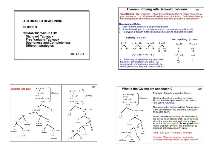
KB - AR - 13 9ai Proof Method: By Refutation. Show by construction that no model can exist for given sentences . i.e. all potential models are contradictory. Do this by following the consequences of the data and showing that they all lead to a contradiction.

Theorem Proving with Semantic Tableaux

Non - splitting (α rules): Splitting ( β rules): Development Rules:

• 1. Start from the givens in a single initial branch
• 2. A tree is developed s.t. sentences in each branch give a partial model
• 3. Two types of branch extension using Non-splitting and Splitting rules:

¬(A → B ) A ¬B A ∧ B A B ¬(A ∨ B ) ¬A ¬B ¬¬A A (¬(A ↔B) ≡ ¬A ↔B ) A B A ∨ B ¬A ¬B ¬ ( A ∧ B) ¬ A B A → B A B ¬A ¬B A ↔B

• 4. Rules may be applied in any order and

branches developed in any order. All sentences in a branch must eventually be developed unless they lead to contradiction. 9aii Example (see ppt): ¬¬e e ¬ (a ∧ w ) p ¬ a ¬ w i a ¬ ¬ w m ¬ e ¬ i∧ ¬ m ¬ i ¬ m ¬ e ¬ i∧ ¬ m ¬ i ¬ m ¬¬e e ¬ e ¬ i∧ ¬ m ¬ i ¬ m i a ¬¬ w m p ¬ (a ∧ w ) ¬ a ¬w Givens a ∧ w → p i ∨ a ¬ w →m ¬ p e → ¬ i∧ ¬ m a ∧ w → p i ∨ a ¬ w →m ¬ p e → ¬ i∧ ¬ m Givens 9aiii Example: There is a model of Givens The branch ending in w does not close. All data has been processed in the branch. (It is called saturated.) The assumption that a model of Givens exists is not contradicted; the branch is consistent and called open. In fact, a model (valuation) can be read from the literals in an open branch. Each positive atom that occurs is assigned true and each atom that occurs negated is assigned false. Atoms that don't occur in the branch can be assigned arbitrarily, usually false. Here: a, e, p, w =True and i, m=False. Question: Why can no atom occur both positively and negatively in an open branch?

What if the Givens are consistent?

¬¬e e ¬ e ¬ i∧ ¬ m ¬ i ¬ m i a ¬¬ w m p ¬ (a ∧ w ) ¬ a ¬w w a ∧ w → p i ∨ a ¬ w →m e → ¬ i∧ ¬ m Givens

9aiv Semantic Tableaux Introduction (1) Brief History: Semantic tableaux were introduced in 1954 by Beth. Both the standard method and free variable methods were automated in 1985. A clausal form of the free variable method (see Slides 10) called Model Elimination, is based on earlier work of Kowalski and Loveland in 1970. They developed Model Elimination as a resolution refinement not a tableau method, but it was later related to tableau methods from 1990 onwards. The TABLEAUX Workshops (now part of IJCAR) are devoted to tableaux and their extended forms and related theorem proving methods. The initial branch of a semantic tableau contains the given sentences that are to be refuted. Note that the sentences do not need to be translated into clausal form. Because the tableau method is refutation based, to show some data D implies conclusion C one needs to negate the conclusion and derive a contradiction from the union of D and ¬C. Reasoning progresses by making assertions about the satisfiability of sub-formulas based on the satisfiability of the larger formulas of which they are a part. For instance, the α-rules (slide 9ai) can be read as "if α is in a branch and there is a model of the sentences in the branch, then there is a model of the sentences in the branch extended by α1 and α2" and the β-rules as "if β is in a branch and there is a model of the sentences in the branch, then there is a model of either the sentences in the branch extended by β1, or the sentences in the branch extended by β2", where α1, α2/β1, β2 are the two sub-formulae of the rules. If X and ¬X are in the branch then the sentences in the branch are clearly inconsistent and the branch is said to be closed. If all branches in a tableau are closed (when the tableau is also said to be closed), then there are no possible consistent derivations of sub-formulas from the initially given sentences, and these sentences are unsatisfiable. 9av Semantic Tableaux Introduction (2) Two examples of closed propositional tableaux are given on slide 9aii, illustrating that there can be differently sized tableaux for the same set of initial sentences. For propositional sentences the development of a tableau will always terminate as there is no need to develop a sentence in a branch more than once – to do so would duplicate

• ne or more sub-formulas or atoms in that branch, which adds no information to the
• branch. However, every sentence in a branch must be developed in it.

A fully developed (or completed) branch is called open if it is not closed, and similarly the tableau. A fully developed open branch will yield a model of the initial data. See slide 9aiii for an example of a fully developed propositional tableau with an open brnach and the corresponding model and 9evi for a proof that a model can be found. 9bi

The invariant property SATISFY:

• Each tableau extension rule maintains satisfiability:

The property SATISFY is used to show Soundness of the tableau method (see Slides 9e). Informally, suppose the givens were satisfiable, then by SATISFY at each step

• ne branch will remain satisfiable. But if the tableau closes, then all branches

are unsatisfiable, so can conclude that givens cannot be satisfiable. e.g. If M is a model of a branch including i ∨ a, then M must assign true to at least one of i or a. Hence at least one of the two extended branches is still satisfied by M.

• A branch that contains both X and ¬ X is unsatisfiable and can be

closed by the closure rule. if the sentences in a branch are satisfiable and a rule is applied, then the new sentences in at least one descendant branch are satisfiable 9bii Soundness and Completeness Statements for Tableaux: The soundness theorem for tableaux states that “if a set of sentences S is consistent, then the tableau developed from S will not (fully) close”. Or, equivalently, "if the tableau developed from sentences S closes, then S is inconsistent". The completenss theorem for tableaux states that “if a set of sentences S is unsatisfiable, then it is possible to find a fully closed tableau derived from them”. The soundness theorem is a consequence of the property (SATISFY), which guarantees that the development rules maintain consistency in at least one descendant

• branch. Informally, therefore, if the original sentences are satisfiable, not all branches

can close. Proofs of both properties are in Slides 9e. First Order Tableaux (Standard Version) There are two kinds of quantifier rules for tableaux; the standard rules for universal- type quantifiers (either ∀ or ¬∃ ) are similar to the usual ∀−elimination rule for natural deduction. That is, occurrences of the bound variable in the scope of the quantifier may be replaced by any term in the language, including terms involving

• ther universally bound variables at the same outer level as (and hence in the scope
• f) the quantifier being eliminated. e.g.∀x∀y.P(x,y) could become ∀y.P(f(a),y) or

even ∀y. P(y,y). The problem with this form of the rule is that the substitutions have to be guessed. (See example on 9cii.) These rules are not often used in theorem provers (although they may be used in proofs about tableau provers). Instead, free variable rules are used. (Notes continued on 9div.)

9ci In this standard version of the γ rules, each ∀ sentence in an open branch B should eventually be used for every term that can be constructed from constants and functors appearing in the branch Question: So you forsee any problems with these rules? Example from 9cii: from ¬∃y (pr(y)∧div(y,n)) obtain ¬(pr(n) ∧div(n,n)) Substitute constant n for variable y, or ¬(pr(f(g(n))) ∧div(f(g(n)),n)) Substitute term f(g(n)) for variable y Two different instances are used, but it could be many more

Rules for universal quantifiers

There are two versions of rules for dealing with ∀ (called γ rules): Standard version (mostly used only in proofs of tableau properties) Free variable version (see slide 9ciii) Standard Universal Rules ∀x P[x] ¬∃x P[x] | | P[t1] ¬ P[t1] where t1 is a ground term from the language of the branch. e.g. ∀x P(x,f(x) ) is in a branch B ⇒ P(s,f(s) ) and also ⇒ P(g(s),f(g(s)) ) where s is a constant and g is a functor used in B (1) div(x,x), (2) less(1,n), (3) div(u,w) ∧ div(w,z) → div(u,z) (4) ¬(div(g(x),x) ∧ less(1,g(x)) ∧ less(g(x),x) ) → pr(x) (5) less(1,x)∧less(x,n)→div(f(x),x)∧pr(f(x)) (6) ¬∃y (pr(y)∧div(y,n)) 9cii div(n,n) ¬less(1,g(n) (6) ¬(pr(n) ∧div(n,n)) (guess n is a good value for y) (4) ¬¬(div(g(n)n) ∧ less(1,g(n)) ∧ less(g(n),n)) div(g(n)n), less(1,g(n)), less(g(n),n) pr(n) div(f(g(n)), g(n)) pr(f(g(n)) ¬ (pr(f(g(n)) ∧div(f(g(n)),n)) ¬ div(f(g(n)),n) ¬(less(1,g(n) ∧ less(g(n),n)) ¬pr(f(g(n)) (5) (6) ¬less(g(n),n) (Use (3) next) ¬pr(n) ¬div(n,n) (1) Guess f(g(n)) is a good value for y in (6) A closed tableau using the Standard γ γ γ γ rules: variables are x,u,w,z and universally quantified; 1, n are constants Example (see ppt) 9ciii

• In a free variable tableau the CHOICE of substitution in a γ-rule application is

delayed until closure.

• The closure rule applies unification to the matching formulas to find a

substitution of free variables to achieve complementarity. The bindings are then applied to all occurrences of the free variables in the tableau

• May apply the rule to a sentence many times (each with a fresh free variable)

REMEMBER: Wherever a free variable (x1 say) occurs in the tableau, it must be bound to the same term (if it is bound at all).

Free Variable Rules for Universal Quantifiers

Standard tableau rules for universal quantifiers have one main problem:

• guessing what to substitute for bound variables (of universal type)

In clausal reasoning resolution replaced guessing substitutions. Free variable rules improve on standard rules by delaying γ rule substitutions. Free variable γ γ γ γ rules ∀x P[x] ¬∃x P[x] | | P[x1] ¬ P[x1] where x1 is a new free variable in the tableau e.g. ∀x P(x,f(x) ) ⇒ P(x1,f(x1) ) (x1 is new to tableau) (1) div(x,x), (2) less(1,n), (3) div(u,w) ∧ div(w,z) → div(u,z) (4) ¬(div(g(x),x) ∧ less(1,g(x)) ∧ less(g(x),x) ) → pr(x) (5) less(1,x)∧less(x,n)→div(f(x),x)∧pr(f(x)) (6) ¬∃y (pr(y)∧div(y,n)) 9civ ¬(pr(y1) ∧div(y1,n))⇒¬(pr(f(g(n)))∧div(f(g(n)),n)) div(g(x1),x1) ∧ less(1,g(x1)) ∧ less(g(x1),x1) ⇒div(g(n),n) ∧ less(1,g(x1)) ∧ less(g(n),n) pr(x1)⇒pr(n) div(f(x2), x2)⇒div(f(g(x1),g(x1)) pr(f(x2)) ⇒pr(f(g(x1)) ⇒div(f(g(n),g(n)) pr(f(g(n)) ¬ less(x2,n) ⇒ ¬less(g(x1),n) ¬ less(1,x2) x2==g(x1) ¬ pr(y2) ¬ div(y2,n) ⇒¬div(n,n) y2==n x3==n div(x3,x3)

Example using Free Variable Universal quantifier rules (ppt)

x1==n y1==f(g(n)) ¬ pr(y1) ¬ div(y1,n) ⇒¬div(f(g(n),n) div(u1,z1) ⇒div(f(g(n)),n) ¬div(w1,z1) ⇒¬div(g(n),z1) ¬ div(u1,w1) u1==f(g(n)) w1==g(n) z1==n

9di Standard (∃ ∃ ∃ ∃) ) ) ) Quantifier rules (δ rules): ∃xP[x] ¬∀xP[x] | | P[a] ¬P[a] where a is a new constant symbol not occurring in the tableau (*) (also called a parameter). e.g. ∀y ∃xP(x,y,y) ⇒ ∃xP(x,b,b) (by ∀ rule) (say b occurs already in the tableau) ⇒ P(c,b,b) (by ∃ rule) (where c is new to the tableau)

Standard Rules for Existential Quantifiers

(*) – in fact, the parameter only needs to be new to the branch). Note: the result of using the standard quantifier rules (both γ and δ) is always a sentence - all variables are bound by a quantifier Think of the rule as "giving a name to the x that maks P[x] true" (eg c in the example) It has to be new, as all that is known about the object c is that P[c} holds. It turns out that with the proviso on the new name the δ-rules obey SATISFY 9dii

Free variable Rules for Existential Quantifiers

Free variable δ δ δ δ rules ∃xP[x] ¬∀xP[x] | | P[a] ¬P[a] where "a" is a term new to the tableau. It is dependent on the free variables occurring in ¬∀xP[x]

• r ∃xP[x] and is a functor of those variables.

If no free variables occur in ¬∀xP[x] or ∃xP[x] then "a" is a new constant, just as in the standard δ-rules. e.g. ∃xP(x,a) ⇒ P(d,a) (no free variables in ∃xP(x,a) so replace by a constant) ∀y,w ∃xP(x,y,w) ⇒ ∃xP(x, y1,w1) (by ∀ rule) (free variables y1,w1) ⇒ P(f(y1,w1), y1,w1) (by ∃ rule) (x is dependent on y1, w1) (functor f is new to the tableau) Can still think of this rule as giving a name to the x that makes P(x, y1,w1) true - but because y1 and w1 could take any value, the name should be different for each combination of values for y1 and w1. eg if y1==a / w1==b, the name for x is f(a,b); if y1==b /w1==a the name for x is f(b,a) It is a uniform structure for the name replacing x, whatever y1 and w1 are bound to. It turns out that with the proviso on the new name the γ-rules obey SATISFY The rules are sometimes called "run-time Skolemisation" (see notes in 9div/v) (2) (∀v[Qxv → Rxg(v)]) → Px (3) Sx → ¬Tg(x)f(y) (4) (Txy → Rxy) → Kxy (5) Qf(z)y ∧ Kzx → Rxg(y) (1) Sa (6) ∀w ¬Pw 9diii Sa ¬Pw1⇒¬Pf(z3) ⇒¬Pf(g(x4) ) ⇒ ¬Pf(g(a) ) ¬(Tx1y1 → Rx1y1) ⇓ ¬(Tz3f(z3) → Rz3f(z3)) Tz3f(z3) ¬Rz3f(z3) Kx1y1 Px2 x2==w1 ¬∀y[Qx2y → Rx2g(y)] ⇓ ¬∀v[Qw1v → Rw1g(v)] ∃v[Qw1v ∧ ¬Rw1g(v)] Qw1h(w1) ¬Rw1g(h(w1)) Rx3g(y3) x3==w1 y3==h(w1) ¬Qf(z3)y3 ⇓ ¬Qf(z3)h(w1) w1==f(z3) ¬Kz3x3 ⇓ ¬Kz3w1 ⇓ ¬Kz3f(z3) x1==z3 y1==f(z3) ¬Sx4 ¬Tg(x4)f(y4) z3==g(x4) y4==z3 x4==a Example using free variable rules (see ppt) Variables x,y,z in (2)-(6) are universally quantified. a is a constant. Work from L to R. Imagine guessing the binding for w1: w1==f(z3)==f(g(x4))==f(g(a)) Free Variable First Order Tableaux When free-variable rules are used for dealing with ∀ sentences, the substituted term is a fresh variable - think of it as a place-holder until a suitable term can be decided. (For this reason, free variables are also sometimes called Unknowns.) A global binding environment for a tableau is maintained, which records eventual bindings to free variables. This is analogous to the procedure in Prolog execution (which can, in fact, be viewed as a particular free-variable tableaux development for Horn clauses). It is as though each universal sentence is replaced by one or more potential instances, where the exact substitutions are still to be decided. Use of the free variable ∀ rule applied to ∀x∀y.P(x,y) yields P(x1, y1), where x1 and y1 are (fresh) free variables (note there is still the freedom for x1 to be bound to the same term as y1). The occurs check is used when unifying at closure to prevent, for example, x1 subsequently being bound to f(x1), as this would lead to infinite terms. An example of this is a branch containing the pair of literals P(x1,f(x1)) and ¬P(f(x2),x2). Unification to close the branch would require to unify {x1=f(x2), f(x1)=x2}, but the unification algorithm will fail, as after setting the substitution x1==f(x2) the second equation becomes f(f(x2))=x2, which will fail the occurs check. Existential-type quantifiers are treated to a Skolemisation process (see slides 9di/ii). For the standard rules the existential rule results in a new constant being introduced, for the free- variable rules it may result in a new (Skolem) function term whose arguments are the free variables in the sentence in the scope of the ∃. 9div

1) It is often easier to initially Skolemise sentences and thus eliminate existential-type quantifiers from the data. (See optional slides 3 for more information. ) The free variable existential rules are sometimes called "run-time Skolemisation" as their effect is similar to Skolemisating at the start. 2) Each existential-type sentence in a branch B is developed once in each branch below B. eg in clause (4) in 9cv "g" is a Skolem term Original sentence: ∀x ∃y [¬(div(y,x) ∧ less(1,y) ∧ less(y,x) ) → pr(x)] becomes ∀x [¬(div(g(x),x) ∧ less(1,g(x)) ∧ less(g(x),x) ) → pr(x)] 9dv Some observations about the Tableaux quantifier rules 2) To develop tableaux systematically, branches are expanded up to a maximum number of applications of γ-rules. If there is no closure and more steps available then the limit is increased. 1) When using the standard rules, for each ∀-type sentence there should be one instance in each (open) branch in which it occurs for each substitution of terms constructed from functors and constants in the branch. Every instance has no unbound variable occurrences and is a sentence. 3) In order to maintain the property of a single binding to any free variable throughout the tableau, bindings are propagated as they are found by unification using the closure rule. γ γ γ γ-rules: δ δ δ δ-rules: There is a potentially infinite number of instances if a functor occurs in the branch. When using free variable rules, can often improve on this requirement - a completely unbound instance of a ∀-type sentence captures many potential instances. Note the variables are called "free" because until they are bound they can have any value in a possible interpretation. 9dvi

Strategies for Developing Tableaux

Systematic: Apply α rules and δ rules Apply γ rules up to a limit Apply splitting rules Why do we need a limit? Apply closure where possible

• r

at fixed intervals For standard ∀rules the limit is usually either i) the total number of applications, or ii) the size of the substituted terms (eg "a" is 1, "f(a)" is 2, "f(a,b)" is 3 etc. For free variable ∀rules the limit may be either i) the total number of free variables introduced, or ii) the total number of γ−rule applications, or iii) a limit on the number of γ−rule applications for each sentence in a branch 9dvii

Heuristics for Developing Tableaux

Extend the rules for A ∧/∨ B to deal with more than one operator of the same kind eg ¬on(x1,z1) ∨ g(x1) ∨ ¬g(z1) gives 3 branches by using the β-rule for ∨ ¬ P(a) ∀x[P(x) ∨ Q(x)] P(a) Q(a) Combine ∀ rule with a splitting rule and possibly closure ∀ + "∨" splitting + closure + choosing 'a' to substitute for the bound variable x. Use splitting rules that will close more than one branch (reduces branching) eg If a branch contained on(a,b) and ¬g(a) then using ¬on(x1,z1) ∨ g(x1) ∨ ¬g(z1) leads to one open branch containing ¬g(b) This can work for standard or free variable tableaux 9dviii Constructing Free Variable Tableaux When deciding on closures in a free variable tableau, you may do it in one of two extreme ways, which could be called "unify as you go", or "unify at the end". All free-variable tableaux on Slides 9

• 11 are constructed using unify-as-you-go. In this kind of construction, whenever a closure is made

that requires a binding to be made to one or more free variables, the substitution is applied to all

• ccurrences in the tableau of those newly bound variables. This guarantees consistency of the

bindings during tableau construction as it enforces the requirement that only one binding may be made to any free variable. The propagation is shown on the slides by an arrow (⇒ or ⇓). This approach is useful for most applications, especially those using data structures, when it may be necessary for a piece of data to be used many times. It has given rise to many different refinements for clausal data. See Slides 10/11. Branches of a tableau may be developed in any order, although usually we use left to right which allows some useful heuristics to be applied; different development

• rders result in different propagation orders and often a different tableau.

In this kind of construction it can be shown that it is unnecessary to put two unconstrained unbound variants of a universal sentence in a branch. However, as soon as such a variant is (even partially) bound, then there is scope for a second variant. eg after applying the ∀ rule to ∀x[P(f(x)) ∨ Q(x)], consider the branch including P(f(x1)); there is no need to use the sentence again as it would result in P(f(x2)), with both x1 and x2 unbound. If later P(f(x1)) happened to be used in closure, binding x1 to a (say), then sibling branches beneath P(f(x1))⇒P(f(a)) could use a second instance P(f(x2)), where the binding of x2 could be constrained to be different from a. This is analogous in not requiring development of a ground sentence in a branch more than once. The alternative method of unify-at-the-end is shown and briefly discussed in the OPTIONAL Appendix 2. In this construction, it is noted when a branch can close and what the corresponding binding is, but no propagation takes place. When every branch is potentially closed the possible substitutions are combined. If they do not successfully combine then alternative closures in one or more branches are sought. The approach is useful if it is known that one (or only a few) occurrences

• f a piece of data will be needed.

9ei

The Standard Tableau Method is Sound

A closed tableau for S implies that S is unsatisfiable

• First show that each tableau extension rule maintains SATISFY:

if the sentences in a branch are satisfiable and a rule is applied, then the new sentences in at least one descendant branch are satisfiable.

• eg: the rule for →: If A → B is in a branch X and there is a model for the

sentences in X, then this model at least makes A false or B true. Hence the same model will ensure satisfiability in one of the two extension branches.

• eg: the rule for ∀:

Suppose ∀x P[x] occurs in a branch B and M is a model for sentences in B. Then if P[t] is added and t is aready interpreted in M then M is still a model;

• therwise, M can be extended by interpreting t as some domain element and still

remain a model. (If data is Skolemised at the start then Sig(S) is known and the first case always applies.)

• Other cases are similar (see 9eii).
• (SATISFY) implies that satisfiable initial sentences can never lead to a fully

closed tableau, as there is always a branch with a model which must be open. (Formally use an induction argument on depth of the tableau.)

• Therefore a fully closed tableau indicates unsatisfiability of the initial sentences.

9eii Proving the Soundness of Tableau: The tableau soundness proof relies on the SATISFY property on Slide 9bv. The cases for boolean operators are all simple and similar to the case given on Slide 9ei. For the standard ∀ case, the argument on 9ei is justified as follows. As in resolution, it is simplest to assume the domain is non-empty (else there are complications). Therefore, assume the domain of M is non-empty. The assignment for t will either already be made in M, or, if t is new and no assignment for t is yet made in M, then t can be any domain

• element. Either way M will remain a model since, in M, P[x] is true for every x in the

domain. In case x is captured by another universal quantifier, as in ∀x,u. P(x,u) becoming ∀u.P(u,u), then since ∀u. P(x,u) is true in M for every domain element substituted for x, in particular, for any domain element substituted for x it follows that P(x,x) is true in M, which is what ∀u P(u,u) is true means. For the standard ∃ case, one can either include in the signature additional parameters to be used as needed (and which are similar to Skolem constants), or introduce new names as the need arises. In both cases it is assumed that M does not have an assignment for the name t introduced by the rule. Since ∃x.P[x] is true, P[a] must be true for some element a in the domain of M. The assignment for the new name t can be the witness a. The cases for the free variable ∀ and ∃ rules are considered on 9evii. The proof uses the following notion: A branch is saturated if all possible development rules have been applied to the sentences in the branch. e.g. for a β-rule, if β1 op β2 belongs to the branch then either β1 or β2 belongs to the branch. Proof of Tableau Soundness To show: If a closed tableau is developed from S then S is unsatisfiable. The proof uses induction on the completed depth of a tableau (defined next). A tableau is completed up to depth n if each branch is either closed (after ≤ n steps), saturated and open (after ≤n steps), or neither and of length = n steps. (Note that a branch that becomes closed at the nth step was not satisfiable at the n-1th step, as it must include two complementary formulas.) Lemma: Let S be a satisfiable set of sentences. Forall n≥ ≥ ≥ ≥0, P(n) holds, where P(n) states that if a tableau T is completed up to depth n using S then T has at least one satisfiable and open branch. Proof (by induction on completed depth): Assume that S is satisfiable. Then S does not contain a sentence A and its negation ¬A. Base Case (n=0). S is satisfiable. Hence the initial branch after no steps is open and P(0) holds. Induction Step (n>0). Assume as induction hypothesis (IH) that if a tableau is developed from a satisfiable set of sentences S, and every branch is completed up to depth k, 0≤k<n, then that tableau has at least one satisfiable and open branch. Let T be a tableau developed from S and completed up to depth n. Either: (i) all branches are closed (not possible by assumption of IH as it would require all branches to be consistent after n-1 steps), or saturated at depth n-1, whence the Lemma holds, or (ii) consider the reduced tableau T ', formed by undoing any step that lengthened a branch to depth n, which is therefore completed up to depth n-1. By (IH) T ' must have some open and satisfiable branch that has been developed to form T. Consider that branch. According to SATISFY at least one branch resulting from that step is open, leading to an open branch in T. Hence by induction we conclude P(n). Finally, if S leads to a closed tableau, then we conclude S is not satisfiable, since a closed tableau has no open branch. 9eiii

The standard tableau method is Complete

For unsatisfiable S a closed tableau for S exists. 9eiv

• Assume S is unsatisfiable and uses language L augmented with a set ∆ of

parameters for use in δ rule applications.

• Apply rules in a systematic and fair way (possibly by contemplating γ−rule

applications for an "infinite" number of times), to obtain a maximally developed saturated tableau, in which all possible applications of the α, β, δ, γ rules are made in all branches. For any branch, all applications of the ∀ rule for terms using L and parameters used in the branch should be made. e.g. can interleave the α, β, δ rules with a finite number of applications of the γ γ γ γ- rule, as on slide 9dii eg if p ∧ q is in a branch B then both p and q are also in B

• Suppose such a maximal tableau doesn't close, then at least one (possibly

infinite) branch B is open (ie it does not contain X and ¬X) and a model of the sentences in B can be constructed based on the literals occurring in B. (See slides 9ev to 9evii.)

• Therefore, if S is unsatisfiable and hence has no model, the assumption is

false and applying the tableau rules to S leads to a closed tableau.

9ev Example of a Saturated Tableau (ppt) Given: b(c) ∃y.on(c,y) ¬b(x)∨¬g(x) ¬on(x,z)∨g(x)∨ ¬g(z) Extensions by any other instances (4 possibilities in all) duplicate at least one literal in the remaining open branch. Such extensions are unnecessary. Exercise: Check this is the case. ∃y.on(c,y) b(c)

• n(c,d)

¬b(c) ¬g(c) g(c) ¬g(d) ¬on(c,d)

• Domain of H-model in the open

branch = {c,d}

• The atoms are on(c,d), b(c), so

these are True.

• All other atoms are false:
• n(c,c), on(d,d), on(d,c), b(d), g(c),

g(d). Check:

• Clearly b(c) and ∃y.on(c,d) are true.
• For each x, g(x) is false so

¬b(x)∨¬g(x) is true.

• For z = c, ¬on(x,z)∨g(x)∨ ¬g(z) is

true as g(c) is false.

• Similarly for z=d.

(Variables x,z are universally quantified and parameter is d)

Constructing a Model from an open branch in a Saturated Tableau

9evi

• A H-interpretation is constructed with domain the set of terms built from

symbols occurring in L+∆', such that atoms in B are assigned true and all other atoms are assigned false. ∆' is the subset of ∆ occurring in sentences in B

• Let S be the set of initial sentences using language L and parameters ∆.
• Suppose a standard tableau has been fully developed from initial sentences

S, as described on Slide 9eiv, and that there is a saturated open branch B.

• Let T be the set of sentences in B and M be a first order H-interpretation of

T with domain terms built from symbols in T and constructed as follows: Each atom in T is true in M; all other atoms are false in M.

• We show M is a model of T.
• Suppose not: then some sentence in T is false in M.
• Let X be the smallest sized sentence in T s.t. M makes X false.
• Whatever type of sentence X is, its being false leads to a contradiction:

(See next slide ....) 9evii Constructing a Model from an open branch in a Saturated Tableau (contd)

• Let T be the set of sentences in B and M be a first order H-interpretation of T

with domain terms built from symbols in T and constructed as follows: Each atom in T is true in M; all other atoms are false in M.

• Let X be the smallest sized sentence in T s.t. M makes X false.
• X cannot be an atom, by construction.
• eg: case X is ¬ Y (Y atom) : If ¬Y is false in M, then Y is true. But then Y
• ccurs in T and closure would have occurred.
• eg: case X is A ∨ B : If A ∨ B is false in M then both A and B are false in M

and smaller than A ∨ B; but at least one of A or B is in T, contradicting that X is the smallest false sentence in T.

• eg: case X is ∀xP[x] : If ∀xP[x] is false in M then P[t] is false for some domain

element t. But by construction P[t] occurs in T and is smaller than ∀xP[x] (assume size is depth of parse tree of X).

• Other cases are similar.

Soundness: When a free variable tableau closes, there may be free variables in it not yet

• bound. These can be bound (consistently) to any ground term yielding a

ground tableau, which will still close. Then use Soundness of a standard tableau. Completeness (outline): A closed standard tableau may be lifted to a tableau using free variables: Each use of the standard ∀-rule is made into a use of the γ -rule, with a fresh set of variables, and each closure then becomes one or more equations to be solved by unification. Since the tableau is closed, a unifier satisfying the set of equations derived in this way exists and hence a most general unifier (mgu) exists also. This mgu can be obtained by the unification algorithm in one attempt ("unify at the end") or in a distributed attempt, corresponding to the different branch closures ("unify as you go"). 9eviii

Soundness and Completeness of free variable tableaux

9fi

• Uses the original structure of knowledge - no need to convert to clausal

form and so no exponential expansion in presence of ↔ sentences;

• Extends to non-classical logics very easily - most non-classical automated

techniques use tableaux as they can mimic the semantics closely;

• Lends itself to linear reasoning - at each extension step made to a leaf L

use a sentence that closes one branch using L. eg Logic Programming can be seen as tableau development;

• Can incorporate equality - we will see later how tableau incorporate

equality quite naturally

• Free variable tableaux may terminate without closure for satisfiable

sentences, when standard tableaux would be infinite;

• There are many refinements for free variable tableau using clausal data,

which are often derived from resolution refinements. In Slides 10 we'll look at Model Elimination, the basis for many of them.

Benefits of the Tableau Approach

9fii

Summary of Slides 9

• 1. Semantic Tableau methods provide an alternative to resolution for theorem
• proving. They are also based on refutation and for a given set of sentences S

attempt to demonstrate that S can have no models.

• 2. In the ``standard'' tableau method, rules for dealing with universal (∀)

sentences require substitution of ground terms for the bound variable. This is avoided in the ``free variable'' tableau method; instead fresh variables are substituted for bound variables, which are bound on branch closure using unification.

• 3. In the ``unify-as-you-go'' development strategy (the only strategy covered

here) the bindings of free variables are immediately propagated to all

• ccurrences of the variables in the tableau. An alternative is the ``unify-at-the-

end'' development strategy, in which potential bindings for free variables are recorded and on (potential) closure of all branches in the tableau are combined. In effect, the difference between the two strategies is whether to combine unifiers as they are generated, or to wait until all have been generated. 4.The tableau method is sound and complete. The free variable soundness and completeness properties are derived from those of the standard tableau method. 9fiii

• 5. The soundness property of tableau depends on the SATISFY property,

which states that, for a consistent branch, the tableau rules maintain consistency in at least one descendant branch.

• 6. The completeness property depends on the notion of saturation, the

development of a tableau to include all possible applications of each rule in every branch.

• 7. The tableau method has several benefits, including: it uses the original

structure of the data, can be extended to many logics such as modal/temporal logic, can easily incorporate equality, and linear and many other refinements can be defined for the tableau method.

• 8. If a tableau terminates finitely without closing every branch, then a model

can be found for any remaining open branches (possibly a different one for each open branch). The slides showed how to construct the model for standard tableaux. It is also possible to do so for free variable tableaux.

• 9. (OPTIONAL) There are several implementations of the tableau method. The

LeanTap approach uses Prolog and results in a very compact program. It exploits Prolog's use of variables to implement the unfication and propagation

• f free variables.

S ST TA AR RT T

• f

f O OP PT TI IO ON NA AL L M MA AT TE ER RI IA AL L ( (S SL LI ID DE ES S 9 9) )

List of Non-resolution Proving Techniques The LeanTap Theorem Prover

9gi Various different techniques have been considered as suitable alternatives to resolution and clausal form for automated reasoning. These include:

• Relax adherence to clausal form:

Non-clausal resolution (Murray, Manna and Waldinger) Semantic tableau /Natural deduction but with unification ( Hahlne, Manna and Waldinger, Reeves, Broda, Dawson, Letz, Baumgartner, Hahlne, Beckert and many others)

• Relax restriction to first order classical logic: Modal logics, resource logics

(Constable, Bundy,Wallen , D'Agostino, McRobbie,) Add sorts (Walther, Cohn, Schmidt Schauss) Higher order logics (Miller, Paulson) Temporal logic with time parameters (Reichgeldt, Hahlne, Gore) Labelled deduction (Gabbay, D'Agostino, Russo, Broda}

• Heuristics and Metalevel reasoning:

Use metalevel rules to guide theorem provers - includes rewriting, paramodulation (Bundy, Dershowitz, Hsiang, Rusinowitz, Bachmair) Abstractions (Plaistead) Procedural rules for natural deduction (Gabbay) Unification for assoc.+commut. operators (Stickel) Use models / analogy (Gerlenter, Bundy) Inductive proofs, proof plans (Boyer and Moore, Bundy et al) Tacticals / interactive proof / proof checkers, Isabelle (Paulson) Considered in Part II (weeks 5-9 of the course) are Tableaux methods and rewriting for equality.

Non-Resolution Theorem Proving

9gii

LeanTap: A Free Variable Tableau Theorem Prover

%prove(currentFormula,todo,branchLits,freevars,maxvars) %Conjunction case (alpha rule) prove((A,B),UE,Ls,FV,V) :- !, prove(A,[B|UE],Ls,FV,V). %Disjunction case - split (beta rule) prove((A;B),UE,Ls,FV,V) :- !, prove(A,UE,Ls,FV,V), prove(B,UE,Ls,FV,V). %Universal case - keep data all(X,Fm) prove(all(X,Fm),UE,Ls,FV,V) :- !, \+ length(FV,V),copy_term((X,Fm,FV),(X1,Fm1,FV)), append(UE,[all(X,Fm)],UE1), prove(Fm1,UE1,Ls,[X1|FV],V). %Closure case prove(Lit,_,[L|Ls],_,_) :- (Lit = -Neg; -Lit = Neg) -> (unify_with_occurs_check(Neg,L); prove(Lit,[],Ls,_,_)). %Literal not matching case prove(Lit,[N|UE],Ls,FV,V) :-prove(N,UE,[Lit|Ls],FV,V). Formulas are in Skolemised negated normal form (negations next to atoms). nnf(-(-(p=>q)=>(q=>p)), ((p,-q),(q,-p))) nnf(-(((p=>q)=>p)=>p), (((p,-q);p),-p)) nnf(ex(Y,all(X,(f(Y)=>f(X)))), all(X,(-f(s);f(X)))) (The code generates all(X,(f(Y)=>f(X))) as Skolem term s) :- op(400,fy,-),op(500,xfy,&),op(600,xfy,v),

• p(650,xfy,=>), op(700,xfy,<=>).

nnf(Fml,NNF) :- nnf(Fml,[],NNF). nnf(Fm,FV,NNF) :- (Fm = -(-A) -> Fm1 = A; Fm = -all(X,F) -> Fm1 = ex(X,-F); Fm = -ex(X,F) -> Fm1 = all(X,-F); Fm = -(A v B) -> Fm1 = -A & -B; Fm = -(A & B) -> Fm1 = -A v -B; Fm = (A => B) -> Fm1 = -A v B; Fm = -(A => B) -> Fm1 = A & -B; Fm = (A <=> B) -> Fm1 = (A & B) v (-A & -B); Fm = -(A <=> B) -> Fm1 = (A & -B) v (-A & B)),!, nnf(Fm1,FV,NNF). nnf(all(X,F),FV,all(X,NNF)) :- !, nnf(F,[X|FV],NNF). nnf(ex(X,Fm),FV,NNF) :- !, copy_term((X,Fm,FV),(Fm,Fm1,FV)), nnf(Fm1,FV,NNF). nnf(A & B,FV,(NNF1,NNF2)) :- !, nnf(A,FV,NNF1), nnf(B,FV,NNF2). nnf(A v B,FV,(NNF1;NNF2)) :- !, nnf(A,FV,NNF1),nnf(B,FV,NNF2). nnf(Lit,_,Lit). 9giii

9giv LeanTap Prover The LeanTap theorem prover was developed by Bernard Beckert, Joachim Possega and Reiner Hahlne. It was the first ``Lean'' theorem prover, meaning a ``very small Prolog program'' that exploits Prolog unification in clever ways to implement a theorem prover for first order logic. A different prover, but equally good, prover is given in the optional part of Slides 10. It is called LeanCop, and both LeanTap and LeanCop belong to the family of Lean provers. It is always impressive to see how compact a theorem prover in Prolog can be. For simplicity, LeanTap uses formulas in Skolemised Negation Normal Form (NNF). This means that before trying to develop a tableau existential type quantifiers are replaced by Skolem functions and negations are pushed inwards so they are next to atoms; however, no distribution of ∧ over ∨, or ∨ over ∧, is applied. This sentence structure allows to simplify the top level of LeanTap, so only conjunctions and disjunctions, universal quantifers and literals need be considered. (LeanCop uses clausal form, which is a sub-case of NNF – ie distribution of ∨ over ∧ is performed. ) Closure is checked for literals only. The Skolemisation step in `nnf' uses the name of the formula being Skolemised as the new Skolem constant. There are several websites covering LeanTap - just type it into Google and see! 9gv Example queries to run: F= (-h(a), all(X,(f(X);h(X))),all(Z,(-g(Z);-f(b))), all(Y,(-f(Y);-h(b))),all(X,(g(X);-f(X)))), prove(F,[],[],[],4) nnf(-(-e)&(a & w =>p)&(i v a)& -p&(e =>-i & -m)&(-w =>m), F), prove(F,[],[],0)

• 1. Add write instructions so that information about the structure of the tableau is printed
• ut, including closure.
• 2. Explain details of universal and closure cases of prove and existential case of nnf.
• 3. Run other examples covered in slides and exercises.

What improvements could be made? a) add a loop check. Note that (for example) h(X) and h(Y) do not form a loop - so must be careful to match terms identically. b) add a higher level predicate prove1 that calls prove recursively, each time increasing the freevars limit by 1. c) limit the depth of each branch instead of the number of freevars. 9gvi More Notes about LeanTap The interesting cases in the program are for universal quantifiers and literals. i) Case all(X,Fm): Note first that a limit is put on the total number of free variables used in the tableau (argument maxvars). If this is not reached then a copy of the formula Fm is made in which the current free variables are not copied, so they are preserved across the tableau. Bound variable X occurrences are copied throughout. ii) Case Lit in Fm: Either the literal causes closure by unification (with the occurs check in place) with a complementary literal in branchLits, or it does not. In the latter case the Lit is added to branchLits. Conversion to NNF is carried out recursively as on Slide 9giii. The existential case ex(X,Fm) introduces a Skolem term in a clever way. It instantiates X with the formula Fm. Thus each unique exists term introduces a different Skolem formula, which is dependent on the free variables in the formula Fm.