
SLIDE 1
http://www.ugrad.cs.ubc.ca/~cs314/Vjan2016
Hidden Surfaces / Depth Test
University of British Columbia CPSC 314 Computer Graphics Jan-Apr 2016 Tamara Munzner
2
Hidden Surface Removal
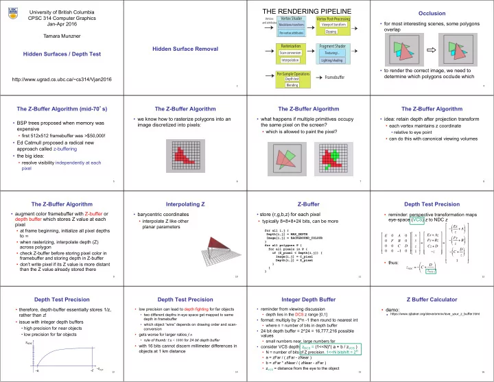
THE RENDERING PIPELINE
Vertex Shader Vertex Post-Processing Rasterization Per-Sample Operations Framebuffer
Vertices and attributes Modelview transform
Interpolation
Per-vertex attributes Clipping Viewport transform
Scan conversion
Fragment Shader
Texturing/... Lighting/shading Depth test Blending
4
Occlusion
- for most interesting scenes, some polygons
- verlap
- to render the correct image, we need to
determine which polygons occlude which
5
The Z-Buffer Algorithm (mid-70’s)
- BSP trees proposed when memory was
expensive
- first 512x512 framebuffer was >$50,000!
- Ed Catmull proposed a radical new
approach called z-buffering
- the big idea:
- resolve visibility independently at each
pixel
6
The Z-Buffer Algorithm
- we know how to rasterize polygons into an
image discretized into pixels:
7
The Z-Buffer Algorithm
- what happens if multiple primitives occupy
the same pixel on the screen?
- which is allowed to paint the pixel?
8
The Z-Buffer Algorithm
- idea: retain depth after projection transform
- each vertex maintains z coordinate
- relative to eye point
- can do this with canonical viewing volumes
9
The Z-Buffer Algorithm
- augment color framebuffer with Z-buffer or
depth buffer which stores Z value at each pixel
- at frame beginning, initialize all pixel depths
to ∞
- when rasterizing, interpolate depth (Z)
across polygon
- check Z-buffer before storing pixel color in
framebuffer and storing depth in Z-buffer
- don’t write pixel if its Z value is more distant
than the Z value already stored there
10
Interpolating Z
- barycentric coordinates
- interpolate Z like other
planar parameters
11
Z-Buffer
- store (r,g,b,z) for each pixel
- typically 8+8+8+24 bits, can be more
for all i,j { Depth[i,j] = MAX_DEPTH Image[i,j] = BACKGROUND_COLOUR } for all polygons P { for all pixels in P { if (Z_pixel < Depth[i,j]) { Image[i,j] = C_pixel Depth[i,j] = Z_pixel } } }
12
Depth Test Precision
- reminder: perspective transformation maps
eye-space (VCS) z to NDC z
- thus:
E A F B C D −1 " # $ $ $ $ % & ' ' ' ' x y z 1 " # $ $ $ $ % & ' ' ' ' = Ex + Az Fy+ Bz Cz + D −z " # $ $ $ $ $ % & ' ' ' ' ' = − Ex z + A ( ) * + ,
- − Fy
z + B ( ) * + ,
- − C + D
z ( ) * + ,
- 1
" # $ $ $ $ $ $ $ $ $ % & ' ' ' ' ' ' ' ' ' zNDC = − C + D zVCS " # $ % & '
13
Depth Test Precision
- therefore, depth-buffer essentially stores 1/z,
rather than z!
- issue with integer depth buffers
- high precision for near objects
- low precision for far objects
- zeye
zNDC
- n
- f
14
Depth Test Precision
- low precision can lead to depth fighting for far objects
- two different depths in eye space get mapped to same
depth in framebuffer
- which object “wins” depends on drawing order and scan-
conversion
- gets worse for larger ratios f:n
- rule of thumb: f:n < 1000 for 24 bit depth buffer
- with 16 bits cannot discern millimeter differences in
- bjects at 1 km distance
15
Integer Depth Buffer
- reminder from viewing discussion
- depth lies in the DCS z range [0,1]
- format: multiply by 2^n -1 then round to nearest int
- where n = number of bits in depth buffer
- 24 bit depth buffer = 2^24 = 16,777,216 possible
values
- small numbers near, large numbers far
- consider VCS depth: zDCS = (1<<N)*( a + b / zVCS )
- N = number of bits of Z precision, 1<<N bitshift = 2n
- a = zFar / ( zFar - zNear )
- b = zFar * zNear / ( zNear - zFar )
- zVCS = distance from the eye to the object
16
Z Buffer Calculator
- demo:
- https://www.sjbaker.org/steve/omniv/love_your_z_buffer.html