The Matrix Geometric/Analytic Methods for Structured Markov Chains - - PowerPoint PPT Presentation

William J. Stewart Department of Computer Science N.C. State University

The Matrix Geometric/Analytic Methods for Structured Markov Chains

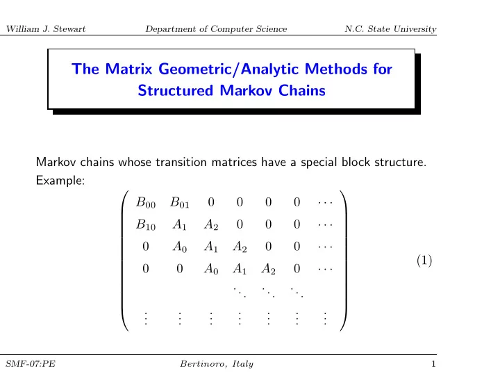
Markov chains whose transition matrices have a special block structure. Example:               B00 B01 · · · B10 A1 A2 · · · A0 A1 A2 · · · A0 A1 A2 · · · ... ... ... . . . . . . . . . . . . . . . . . . . . .               (1)

SMF-07:PE Bertinoro, Italy 1

William J. Stewart Department of Computer Science N.C. State University

Each state can be written as {(η, k), η ≥ 0, 1 ≤ k ≤ K} — ordered by increasing value of η then by increasing value of k. States are grouped into “levels” according to their η value. The block tridiagonal effect: transitions are permitted — between states of the same level (diagonal blocks), — to states in the next highest level (super-diagonal blocks), — and to states in the adjacent lower level (sub-diagonal blocks). Called Quasi-Birth-Death (QBD) processes.

SMF-07:PE Bertinoro, Italy 2

William J. Stewart Department of Computer Science N.C. State University

Example:

5,3

λ

1

λ λ λ λ λ λ λ λ λ λ λ

1 1 1 1 1 2 2 2 2 2 2

γ γ γ γ γ γ γ γ γ γ γ

1 1

γ γ γ γ γ γ γ γ γ

1 1 1 1 1 1 1 1 2 2 2 2 2 2 2 2 2 2

γ γ

1 2

µ µ µ µ µ

0,1 0,2 1,1 1,2 1,3 2,1 2,2 2,3 3,1 3,2 3,3 4,1 4,2 4,3 5,1 5,2

Figure 1: State transition diagram for an M/M/1-type process.

SMF-07:PE Bertinoro, Italy 3

William J. Stewart Department of Computer Science N.C. State University

Transition rate matrix:

B B B B B B B B B B B B B B B B B B B B B B B B B B B B B B B B B B B B B @ ∗ γ1 λ1 γ2 ∗ λ2 ∗ γ1 λ1 µ/2 µ/2 γ2 ∗ γ1 γ2 ∗ λ2 ∗ γ1 λ1 µ γ2 ∗ γ1 γ2 ∗ λ2 ∗ γ1 λ1 µ γ2 ∗ γ1 γ2 ∗ λ2 ∗ γ1 λ1 µ γ2 ∗ γ1 γ2 ∗ λ2 ... ... ... 1 C C C C C C C C C C C C C C C C C C C C C C C C C C C C C C C C C C C C C A

SMF-07:PE Bertinoro, Italy 4

William J. Stewart Department of Computer Science N.C. State University

Block matrices:

A0 = B B @ µ 1 C C A , A2 = B B @ λ1 λ2 1 C C A A1 = B B @ −(γ1 + λ1) γ1 γ2 −(µ + γ1 + γ2) γ1 γ2 −(γ2 + λ2) 1 C C A and B00 = @ −(γ1 + λ1) γ1 γ2 −(γ2 + λ2) 1 A , B01 = @ λ1 λ2 1 A , B10 = B B @ µ/2 µ/2 1 C C A .

SMF-07:PE Bertinoro, Italy 5

William J. Stewart Department of Computer Science N.C. State University

Most common extensions: — block upper Hessenberg (M/G/1-type, solved using the matrix analytic approach) — block lower Hessenberg GI/M/1-type, solved using the matrix geometric approach).

Q = B B B B B B B B B B B B B B B @ B00 B01 · · · B10 B11 A0 · · · B20 B21 A1 A0 · · · B30 B31 A2 A1 A0 · · · B40 B41 A3 A2 A1 A0 · · · . . . ... ... ... ... ... · · · . . . . . . . . . . . . . . . . . . . . . · · · 1 C C C C C C C C C C C C C C C A

SMF-07:PE Bertinoro, Italy 6

William J. Stewart Department of Computer Science N.C. State University

The Quasi-Birth-Death Case When the blocks of a QBD process are reduced to single elements: Q =           −λ λ µ −(λ + µ) λ µ −(λ + µ) λ µ −(λ + µ) λ ... ... ...           . From πQ = 0, we may write −λπ0 + µπ1 = 0, π1 = (λ/µ)π0 In general λπi−1 − (λ + µ)πi + µπi+1 = 0, which gives πi+1 = (λ/µ)πi i = 1, 2, . . .

SMF-07:PE Bertinoro, Italy 7

William J. Stewart Department of Computer Science N.C. State University

Proof by induction: Basis clause, π1 = (λ/µ)π0. From the inductive hypothesis πi = (λ/µ)πi−1 and hence πi+1 = λ + µ µ

• πi −

λ µ

• πi−1 =

λ µ

• πi.

πi = λ µ i π0 = ρiπ0 where ρ = λ/µ. Once π0 is known, the remaining values, πi, i = 1, 2, . . . , may be determined recursively. A similar result exists when Q is a QBD process: — the parameter ρ becomes a square matrix R of order K — the components πi become subvectors of length K.

SMF-07:PE Bertinoro, Italy 8

William J. Stewart Department of Computer Science N.C. State University

QBD process πQ = 0 with Q =               B00 B01 · · · B10 A1 A2 · · · A0 A1 A2 · · · A0 A1 A2 · · · ... ... ... . . . . . . . . . . . . . . . . . . . . .               Let π be partitioned conformally with Q, i.e. π = (π0, π1, π2, · · · ) where πi = (π(i, 1), π(i, 2), · · · π(i, K))

SMF-07:PE Bertinoro, Italy 9

William J. Stewart Department of Computer Science N.C. State University

This gives the following equations π0B00 + π1B10 = π0B01 + π1A1 + π2A0 = π1A2 + π2A1 + π3A0 = . . . πi−1A2 + πiA1 + πi+1A0 = 0, i = 2, 3, . . . In analogy with the point situation, there exists a constant matrix R s.t. πi = πi−1R, for i = 2, 3, . . . (2) The subvectors πi are geometrically related to each other since πi = π1Ri−1, for i = 2, 3, . . . (3) Given π0, π1 and R, we can find all other πi.

SMF-07:PE Bertinoro, Italy 10

William J. Stewart Department of Computer Science N.C. State University

Substituting from Equation (3) into πi−1A2 + πiA1 + πi+1A0 = 0 gives π1Ri−2A2 + π1Ri−1A1 + π1RiA0 = 0 i.e., π1Ri−2 A2 + RA1 + R2A0

• = 0

So find R from

• A2 + RA1 + R2A0
• = 0.

(4) The simplest way: successive substitution. Equation (4) gives A2A−1

1

+ R + R2A0A−1

1

= 0 i.e., R = −A2A−1

1

− R2A0A−1

1

= −V − R2W R(0) = 0; R(k+1) = −V − R2

(k)W,

k = 1, 2, . . . (5)

SMF-07:PE Bertinoro, Italy 11

William J. Stewart Department of Computer Science N.C. State University

Derivation of π0 and π1: The first two equations of πQ = 0 are π0B00 + π1B10 = π0B01 + π1A1 + π2A0 = Replacing π2 with π1R (π0, π1)   B00 B01 B10 A1 + RA0   = (0, 0) (6) which can be solved for π0 and π1 with the condition πe = 1. 1 = πe = π0e + π1e +

∞

• i=2

πie = π0e + π1e +

∞

• i=2

π1Ri−1e = π0e +

∞

• i=1

π1Ri−1e = π0e +

∞

• i=0

π1Rie.

SMF-07:PE Bertinoro, Italy 12

William J. Stewart Department of Computer Science N.C. State University

This implies the condition π0e + π1 ∞

• i=0

Ri

• e = 1.

The eigenvalues of R lie inside the unit circle which means that (I − R) is nonsingular and hence that ∞

• i=0

Ri

• = (I − R)−1.

(7) Normalize the vectors π0 and π1 by computing α = π0e + π1 (I − R)−1 e and dividing the computed subvectors π0 and π1 by α.

SMF-07:PE Bertinoro, Italy 13

William J. Stewart Department of Computer Science N.C. State University

Ergodicity condition for QBD processes: — the drift to higher numbered levels must be strictly less than the drift to lower levels. Let A = A0 + A1 + A2 and πAA = 0. The following condition must hold for a QBD process to be ergodic πAA2e < πAA0e (8) Elements of A2 move the process up a level while those of A0 move it down a level.

SMF-07:PE Bertinoro, Italy 14

William J. Stewart Department of Computer Science N.C. State University

SUMMARY: Matrix geometric method:

• 1. Ensure that the matrix has the requisite block structure.
• 2. Use Equation (8) to ensure that the Markov chain is ergodic.
• 3. Use Equation (5) to compute the matrix R.
• 4. Solve the system of equations (6) for π0 and π1.
• 5. Compute the normalizing constant α and normalize π0 and π1.
• 6. Use Equation (2) to compute the remaining components of the

stationary distribution vector. For a discrete-time Markov chain, replace −A−1

1

with (I − A1)−1.

SMF-07:PE Bertinoro, Italy 15

William J. Stewart Department of Computer Science N.C. State University

Example: We use the following values of the parameters: λ1 = 1, λ2 = .5, µ = 4, γ1 = 5, γ2 = 3. The infinitesimal generator is then given by

Q = B B B B B B B B B B B B B B B B B B B B @ −6 5.0 1 3 −3.5 .5 −6 5 1 2 2 3 −12 5.0 3 −3.5 .5 −6 5 1 4 3 −12 5.0 3 −3.5 .5 ... ... ... 1 C C C C C C C C C C C C C C C C C C C C A

• 1. The matrix obviously has the correct QBD structure.

SMF-07:PE Bertinoro, Italy 16

William J. Stewart Department of Computer Science N.C. State University

• 2. We check that the system is stable by verifying Equation (8). The

infinitesimal generator matrix A = A0 + A1 + A2 =     −5 5 3 −8 5 3 −3     has stationary probability vector πA = (.1837, .3061, .5102) and .4388 = πAA2e < πAA0e = 1.2245

SMF-07:PE Bertinoro, Italy 17

William J. Stewart Department of Computer Science N.C. State University

• 3. We now initiate the iterative procedure to compute the rate matrix
• R. The inverse of A1 is

A−1

1

=     −.2466 −.1598 −.2283 −.0959 −.1918 −.2740 −.0822 −.1644 −.5205     which allows us to compute V = A2A−1

1

=     −.2466 −.1598 −.2283 −.0411 −.0822 −.2603     W = A0A−1

1

=     −.3836 −.7671 −1.0959     .

SMF-07:PE Bertinoro, Italy 18

William J. Stewart Department of Computer Science N.C. State University

Equation (5) becomes R(k+1) =     .2466 .1598 .2283 .0411 .0822 .2603    +R2

(k)

    .3836 .7671 1.0959     and iterating successively, beginning with R(0) = 0, we find R(1) =     .2466 .1598 .2283 .0411 .0822 .2603     , R(2) =     .2689 .2044 .2921 .0518 .1036 .2909     , R(3) =     .2793 .2252 .2921 .0567 .1134 .3049     , · · · Observe that the elements are non-decreasing.

SMF-07:PE Bertinoro, Italy 19

William J. Stewart Department of Computer Science N.C. State University

After 48 iterations, successive differences are less than 10−12, at which point R(48) =     .2917 .2500 .3571 .0625 .1250 .3214     .

• 4. Proceeding to the boundary conditions:

(π0, π1) @ B00 B01 B10 A1 + RA0 1 A = (π0, π1) B B B B B B B B @ −6 5.0 1 3 −3.5 .5 −6 6.0 2 2 3 −12.0 5.0 3.5 −3.5 1 C C C C C C C C A = (0, 0)

SMF-07:PE Bertinoro, Italy 20

William J. Stewart Department of Computer Science N.C. State University

Solve this by replacing the last equation with π01 = 1, i.e., set the first component of the subvector π0 to 1.

(π0, π1) B B B B B B B B @ −6 5.0 1 1 3 −3.5 −6 6.0 2 2 3 −12.0 3.5 1 C C C C C C C C A = (0, 0 | 0, 0, 1) with solution (π0, π1) = (1.0, 1.6923, | .3974, .4615, .9011) Now on to the normalization stage.

SMF-07:PE Bertinoro, Italy 21

William J. Stewart Department of Computer Science N.C. State University

• 5. The normalization constant is

α = π0e + π1 (I − R)−1 e = (1.0, 1.6923)e + (.3974, .4615, .9011)     1.4805 .4675 .7792 1 .1364 .2273 .15455     e = 2.6923 + 3.2657 = 5.9580 which allows us to compute π0/α = (.1678, .2840) and π1/α = (.0667, .0775, .1512)

SMF-07:PE Bertinoro, Italy 22

William J. Stewart Department of Computer Science N.C. State University

• 6. Subcomponents of the stationary distribution:

— computed from πk = πk−1R. π2 = π1R = (.0667, .0775, .1512)     .2917 .2500 .3571 .0625 .1250 .3214     = (.0289, .0356, .0724) and π3 = π2R = (.0289, .0356, .0724)     .2917 .2500 .3571 .0625 .1250 .3214     = (.0130, .0356, .0336) and so on.

SMF-07:PE Bertinoro, Italy 23

William J. Stewart Department of Computer Science N.C. State University

Block Lower-Hessenberg Markov Chains Q =                 B00 B01 · · · B10 B11 A0 · · · B20 B21 A1 A0 · · · B30 B31 A2 A1 A0 · · · B40 B41 A3 A2 A1 A0 · · · . . . ... ... ... ... ... · · · . . . . . . . . . . . . . . . . . . . . . · · ·                 Transitions are now permitted from any level to any lower level. Objective:compute the stationary probability vector π from πQ = 0. π is partitioned conformally with Q, i.e. π = (π0, π1, π2, · · · ) — πi = (π(i, 1), π(i, 2), · · · π(i, K)).

SMF-07:PE Bertinoro, Italy 24

William J. Stewart Department of Computer Science N.C. State University

A matrix geometric solution exists which mirrors that of a QBD process,. There exists a positive matrix R such that πi = πi−1R, for i = 2, 3, . . . i.e., that πi = π1Ri−1, for i = 2, 3, . . . From πQ = 0

∞

• k=0

πk+jAk = 0, j = 1, 2, . . . and in particular, π1A0 + π2A1 +

∞

• k=2

πk+1Ak = 0

SMF-07:PE Bertinoro, Italy 25

William J. Stewart Department of Computer Science N.C. State University

Substituting πi = π1Ri−1 into π1A0 + π1RA1 +

∞

• k=2

π1RkAk = 0 gives π1

• A0 + RA1 +

∞

• k=2

RkAk

• = 0

So find R from A0 + RA1 +

∞

• k=2

RkAk = 0 (9) Equation (9) reduces to Equation (4) when Ak = 0 for k > 2.

SMF-07:PE Bertinoro, Italy 26

William J. Stewart Department of Computer Science N.C. State University

Rearranging Equation (9), we find R = −A0A−1

1

−

∞

• k=2

RkAkA−1

1

R(0) = 0; R(l+1) = −A0A−1

1

−

∞

• k=2

Rk

(l)AkA−1 1 ,

l = 1, 2, . . . In many cases, the structure of the infinitesimal generator is such that the blocks Ai are zero for relatively small values of i, which limits the computational effort needed in each iteration.

SMF-07:PE Bertinoro, Italy 27

William J. Stewart Department of Computer Science N.C. State University

Derivation of the initial subvectors π0 and π1. From the first equation of πQ = 0,

∞

• i=0

πiBi0 = 0 and we may write π0B00+

∞

• i=1

πiBi0 = π0B00+

∞

• i=1

π1Ri−1Bi0 = π0B00+π1 ∞

• i=1

Ri−1Bi0

• = 0,

(10) From the second equation of πQ = 0, π0B01 +

∞

• i=1

πiBi1 = 0, i.e., π0B01 + π1

∞

• i=1

Ri−1Bi1 = 0. (11)

SMF-07:PE Bertinoro, Italy 28

William J. Stewart Department of Computer Science N.C. State University

In matrix form, we can compute π0 and π1 from (π0, π1)     B00 B01 ∞

i=1 Ri−1Bi0

∞

i=1 Ri−1Bi1

    = (0, 0). Once found, normalize by dividing by α = π0e + π1 ∞

• i=1

Rk−1

• e = π0e + π1(I − R)−1e.

For discrete-time Markov chains, replace −A−1

1

with (I − A1)−1.

SMF-07:PE Bertinoro, Italy 29

William J. Stewart Department of Computer Science N.C. State University

Same example as before, but with additional transitions (ξ1 = .25 and ξ2 = .75) to lower non-neighboring states.

2

λ

1

λ λ λ λ λ λ λ λ λ λ λ

1 1 1 1 1 2 2 2 2 2 2

γ γ γ γ γ γ γ γ γ γ γ

1 1

γ γ γ γ γ γ γ γ γ

1 1 1 1 1 1 1 1 2 2 2 2 2 2 2 2 2 2

γ γ

1 2

µ µ µ µ µ

0,1 0,2 1,1 1,2 1,3 2,1 2,2 2,3 3,1 3,2 3,3 4,1 4,2 4,3 5,1 5,2 5,3

ξ ξ ξ ξ ξ ξ ξ ξ ξ

1 1 1 1 1 1

ξ ξ ξ

2 2 2 2 2

Figure 2: State transition diagram for a GI/M/1-type process.

SMF-07:PE Bertinoro, Italy 30

William J. Stewart Department of Computer Science N.C. State University

Q = B B B B B B B B B B B B B B B B B B B B B B B B B B B B B @ −6 5.0 1 3 −3.5 .5 −6 5 1 2.00 2.00 3 −12 5 3 −3.5 .5 .25 −6.25 5 1 4 3.00 −12 5.00 .75 3 −4.25 .5 .25 −6.25 5 1 4 3.00 −12 5.00 .75 3 −4.25 ... ... ...

SMF-07:PE Bertinoro, Italy 31

William J. Stewart Department of Computer Science N.C. State University

The computation of the matrix R proceeds as previously:

A−1

1

= B B @ −.2233 −.1318 −.1550 −.0791 −.1647 −.1938 −.0558 −.1163 −.3721 1 C C A

which allows us to compute

A0A−1

1

= B B @ −.2233 −.1318 −.1550 −.0279 −.0581 −.1860 1 C C A , A2A−1

1

= B B @ −.3163 −.6589 −.7752 1 C C A A3A−1

1

= B B @ −.0558 −.0329 −.0388 −.0419 −.0872 −.2791 1 C C A ,

SMF-07:PE Bertinoro, Italy 32

William J. Stewart Department of Computer Science N.C. State University

The iterative process is

R(k+1) = B B @ .2233 .1318 .1550 .0279 .0581 .1860 1 C C A + R2

(k)

B B @ .3163 .6589 .7752 1 C C A +R3

(k)

B B @ .0558 .0329 .0388 .0419 .0872 .2791 1 C C A

Iterating successively, beginning with R(0) = 0, we find

R(1) = B B @ .2233 .1318 .1550 .0279 .0581 .1860 1 C C A , R(2) = B B @ .2370 .1593 .1910 .0331 .0686 .1999 1 C C A ,

SMF-07:PE Bertinoro, Italy 33

William J. Stewart Department of Computer Science N.C. State University

R(3) = B B @ .2415 .1684 .2031 .0347 .0719 .2043 1 C C A , · · ·

SMF-07:PE Bertinoro, Italy 34

William J. Stewart Department of Computer Science N.C. State University

After 27 iterations, successive differences are less than 10−12, at which point R(27) =     .2440 .1734 .2100 .0356 .0736 .1669     . The boundary conditions are now (π0, π1)   B00 B01 B10 + RB20 B11 + RB21 + R2B31   = (0, 0)

SMF-07:PE Bertinoro, Italy 35

William J. Stewart Department of Computer Science N.C. State University

= (π0, π1) B B B B B B B B @ −6.0 5.0 1 3.0 −3.5 .5 .0610 .1575 −5.9832 5.6938 .0710 2.0000 2.000 3.000 −12.0000 5.0000 .0089 .1555 .0040 3.2945 −3.4624 1 C C C C C C C C A = (0, 0). Solve this by replacing the last equation with π01 = 1. (π0, π1) B B B B B B B B @ −6.0 5.0 1 1 3.0 −3.5 .0610 .1575 −5.9832 5.6938 2.0000 2.000 3.000 −12.0000 .0089 .1555 .0040 3.2945 1 C C C C C C C C A = (0, 0 | 0, 0, 1) Solution (π0, π1) = (1.0, 1.7169, | .3730, .4095, .8470)

SMF-07:PE Bertinoro, Italy 36

William J. Stewart Department of Computer Science N.C. State University

The normalization constant is α = π0e + π1 (I − R)−1 e = (1.0, 1.7169)e + (.3730, .4095, .8470)     1.3395 .2584 .3546 1 .0600 .1044 1.2764     e = 2.7169 + 2.3582 = 5.0751 Thus: π0/α = (.1970, .3383), and π1/α = (.0735, .0807, .1669). Successive subcomponents are now computed from πk = πk−1R.

SMF-07:PE Bertinoro, Italy 37

William J. Stewart Department of Computer Science N.C. State University

π2 = π1R = (.0735, .0807, .1669)     .2440 .1734 .2100 .0356 .0736 .1669     = (.0239, .0250, .0499) and π3 = π2R = (.0239, .0250, .0499)     .2440 .1734 .2100 .0356 .0736 .1669     = (.0076, .0078, .0135) and so on.

SMF-07:PE Bertinoro, Italy 38

William J. Stewart Department of Computer Science N.C. State University

Simplifications occur when the initial B blocks have the same dimensions as the A blocks and when

Q = B B B B B B B B B B B B B B B @ B00 A0 · · · B10 A1 A0 · · · B20 A2 A1 A0 · · · B30 A3 A2 A1 A0 · · · B40 A4 A3 A2 A1 A0 · · · . . . ... ... ... ... ... · · · . . . . . . . . . . . . . . . . . . . . . · · · 1 C C C C C C C C C C C C C C C A

In this case πi = π0Ri, for i = 1, 2, . . . , ∞

i=0 RiBi0 is an infinitesimal generator matrix

π0 is the stationary probability vector of ∞

i=0 RiBi0

— normalized so that π0(I − R)−1e = 1.

SMF-07:PE Bertinoro, Italy 39

William J. Stewart Department of Computer Science N.C. State University

Also, in some applications more than two boundary columns can occur.

Q = B B B B B B B B B B B B B B B B B B B B B B B @ B00 B01 B02 A0 B10 B11 B12 A1 A0 B20 B21 B22 A2 A1 A0 B30 B31 B32 A3 A2 A1 A0 B40 B41 B42 A4 A3 A2 A1 A0 B50 B51 B52 A5 A4 A3 A2 A1 A0 B60 B61 B62 A6 A5 A4 A3 A2 A1 A0 B70 B71 B72 A7 A6 A5 A4 A3 A2 A1 A0 B80 B81 B82 A8 A7 A6 A5 A4 A1 A0 . . . . . . . . . ... ... ... ... ... ... ... ... ... 1 C C C C C C C C C C C C C C C C C C C C C C C A At present, this matrix is not block lower Hessenberg.

SMF-07:PE Bertinoro, Italy 40

William J. Stewart Department of Computer Science N.C. State University

Restructured into the form

B B B B B B B B B B B B B B B B B B B B B B B @ B00 B01 B02 A0 B10 B11 B12 A1 A0 B20 B21 B22 A2 A1 A0 B30 B31 B32 A3 A2 A1 A0 B40 B41 B42 A4 A3 A2 A1 A0 B50 B51 B52 A5 A4 A3 A2 A1 A0 B60 B61 B62 A6 A5 A4 A3 A2 A1 A0 B70 B71 B72 A7 A6 A5 A4 A3 A2 A1 A0 B80 B81 B82 A8 A7 A6 A5 A4 A1 A0 . . . . . . . . . . . . . . . . . . ... ... ... ... ... ... 1 C C C C C C C C C C C C C C C C C C C C C C C A A0 = B B @ A0 A1 A0 A2 A1 A0 1 C C A , A1 = B B @ A3 A2 A1 A4 A3 A2 A5 A4 A3 1 C C A , B00 = B B @ B00 B01 B02 B10 B11 B12 B20 B21 B22 1 C C A , · · ·

SMF-07:PE Bertinoro, Italy 41

William J. Stewart Department of Computer Science N.C. State University

Block Upper-Hessenberg Markov Chains For QBD and GI/M/1-type processes, we posed the problem in terms of continuous-time Markov chains. Discrete-time Markov chains can be treated if the matrix inverse A−1

1

is replaced with the inverse (I − A1)−1. This time we shall consider the discrete-time case. P =              B00 B01 B02 B03 · · · B0j · · · B10 A1 A2 A3 · · · Aj · · · A0 A1 A2 · · · Aj−1 · · · A0 A1 · · · Aj−2 · · · A0 · · · Aj−3 · · · . . . . . . . . . . . . . . . . . . . . .             

SMF-07:PE Bertinoro, Italy 42

William J. Stewart Department of Computer Science N.C. State University

A = ∞

i=0 Ai is a stochastic matrix assumed to be irreducible.

πAA = πA, and πAe = 1. P is known to be positive-recurrent if πA ∞

• i=1

iAi e

• ≡ πA b < 1.

(12) We seek to compute π from πP = π. As before, we partition π conformally with P, i.e. π = (π0, π1, π2, · · · ) where πi = (π(i, 1), π(i, 2), · · · π(i, K)) The analysis of M/G/1-type processes is more complicated than that of QBD or GI/M/1-type processes because the subvectors πi no longer have a matrix geometric relationship with one another.

SMF-07:PE Bertinoro, Italy 43

William J. Stewart Department of Computer Science N.C. State University

The key to solving upper block-Hessenberg structured Markov chains is the computation of a certain stochastic matrix G. Gij is the conditional probability that starting in state i of any level n ≥ 2, the process enters level n − 1 for the first time by arriving at state j of that level. This matrix satisfies the fixed point equation G =

∞

• i=0

AiGi and is indeed is the minimal non-negative solution of X =

∞

• i=0

AiXi. It can be found by means of the iteration G(0) = 0; G(k+1) =

∞

• i=0

AiGi

(k) = 0,

k = 0, 1, . . .

SMF-07:PE Bertinoro, Italy 44

William J. Stewart Department of Computer Science N.C. State University

Once the matrix G has been computed, then successive components of π can be found. From πP = π π(I − P) = 0,

(π0, π1, · · · , πj, · · · ) B B B B B B B B B B B @ I − B00 −B01 −B02 −B03 · · · −B0j · · · −B10 I − A1 −A2 −A3 · · · −Aj · · · −A0 I − A1 −A2 · · · −Aj−1 · · · −A0 I − A1 · · · −Aj−2 · · · −A0 · · · −Aj−3 · · · . . . . . . . . . . . . . . . . . . . . . 1 C C C C C C C C C C C A (13) = (0, 0, · · · 0, · · · ).

The submatrix in the lower right block is block Toeplitz. There is a decomposition of this Toeplitz matrix into a block upper triangular matrix U and block lower triangular matrix L.

SMF-07:PE Bertinoro, Italy 45

William J. Stewart Department of Computer Science N.C. State University

U = B B B B B B B B B @ A∗

1

A∗

2

A∗

3

A∗

4

· · · A∗

1

A∗

2

A∗

3

· · · A∗

1

A∗

2

· · · A∗

1

· · · . . . . . . . . . ... 1 C C C C C C C C C A and L = B B B B B B B B B @ I · · · −G I · · · −G I · · · −G I · · · . . . . . . ... ... 1 C C C C C C C C C A .

Once the matrix G has been formed then L is known. The inverse of L can be written in terms of the powers of G.

B B B B B B B B B @ I · · · −G I · · · −G I · · · −G I · · · . . . . . . ... ... 1 C C C C C C C C C A B B B B B B B B B @ I · · · G I · · · G2 G I · · · G3 G2 G I · · · . . . . . . ... ... 1 C C C C C C C C C A = B B B B B B B B B @ 1 · · · 1 · · · 1 · · · 1 · · · . . . . . . . . . ... 1 C C C C C C C C C A .

SMF-07:PE Bertinoro, Italy 46

William J. Stewart Department of Computer Science N.C. State University

From Equation (13),

(π0, π1, · · · , πj, · · · ) B B B B B B B B B B B @ I − B00 −B01 −B02 −B03 · · · −B0j · · · −B10 UL . . . 1 C C C C C C C C C C C A = (0, 0, · · · 0, · · · )

which allows us to write π0 (−B01, −B02, · · · ) + (π1, π2, · · · ) UL = 0

• r

π0 (B01, B02, · · · ) L−1 = (π1, π2, · · · ) U,

SMF-07:PE Bertinoro, Italy 47

William J. Stewart Department of Computer Science N.C. State University

π0 (B01, B02, · · · ) B B B B B B B B B @ I · · · G I · · · G2 G I · · · G3 G2 G I · · · . . . . . . ... ... 1 C C C C C C C C C A = (π1, π2, · · · ) U

π0 (B∗

01, B∗ 02, · · · ) = (π1, π2, · · · ) U

(14)

B∗

01

= B01 + B02G + B03G2 + · · · =

∞

X

k=1

B0kGk−1 B∗

02

= B02 + B03G + B04G2 + · · · =

∞

X

k=2

B0kGk−2 . . . B∗

0i

= B0i + B0,i+1G + B0,i+2G2 + · · · =

∞

X

k=i

B0kGk−i

SMF-07:PE Bertinoro, Italy 48

William J. Stewart Department of Computer Science N.C. State University

Can compute the successive components of π once π0 and U are known: π0 (B∗

01, B∗ 02, · · · ) = (π1, π2, · · · )

          A∗

1

A∗

2

A∗

3

A∗

4

· · · A∗

1

A∗

2

A∗

3

· · · A∗

1

A∗

2

· · · A∗

1

· · · . . . . . . . . . ...           Observe that

π0B∗

01 = π1A∗ 1

= ⇒ π1 = π0B∗

01A∗ 1 −1

π0B∗

02 = π1A∗ 2 + π2A∗ 1

= ⇒ π2 = π0B∗

02A∗ 1 −1 − π1A∗ 2A∗ 1 −1

π0B∗

03 = π1A∗ 3 + π2A∗ 2 + π3A∗ 1

= ⇒ π3 = π0B∗

03A∗ 1 −1 − π1A∗ 3A∗ 1 −1 − π2A∗ 2A∗ 1 −1

. . .

SMF-07:PE Bertinoro, Italy 49

William J. Stewart Department of Computer Science N.C. State University

In general: πi =

• π0B∗

0i − π1A∗ i − π2A∗ i−1 − · · · − πi−1A∗ 2

• A∗

1 −1,

i = 1, 2, . . . =

• π0B∗

0i − i−1

• k=1

πkA∗

i−k+1

• A∗

1 −1.

First subvector π0 : π0 (B∗

01, B∗ 02, · · · ) = (π1, π2, · · · ) U

(π0, π1, · · · , πj, · · · ) B B B B B B B B B B B B B @ I − B00 −B∗

01

−B∗

02

−B∗

03

· · · −B∗

0j

· · · −B10 A∗

1

A∗

2

A∗

3

· · · A∗

j

· · · A∗

1

A∗

2

· · · Aj−1 · · · A∗

1

· · · A∗

j−2

· · · . . . · · · . . . 1 C C C C C C C C C C C C C A = (0, 0, · · · 0, · · · )

SMF-07:PE Bertinoro, Italy 50

William J. Stewart Department of Computer Science N.C. State University

First two equations: π0 (I − B00) − π1B10 = 0, −π0B∗

01 + π1A∗ 1 = 0.

Second gives π1 = π0B∗

01A∗ 1 −1.

Substitute into first π0 (I − B00) − π0B∗

01A∗ 1 −1B10 = 0

• r

π0

• I − B00 − B∗

01A∗ 1 −1B10

• = 0

Can now compute π0 to a multiplicative constant. To normalize, enforce the condition: π0e + π0 ∞

• i=1

B∗

0i

∞

• i=1

A∗

i

−1 e = 1. (15)

SMF-07:PE Bertinoro, Italy 51

William J. Stewart Department of Computer Science N.C. State University

Computation of the matrix U from

UL = B B B B B B B B B @ I − A1 −A2 −A3 · · · −Aj · · · −A0 I − A1 −A2 · · · −Aj−1 · · · −A0 I − A1 · · · −Aj−2 · · · −A0 · · · −Aj−3 · · · . . . . . . . . . . . . . . . . . . 1 C C C C C C C C C A .

SMF-07:PE Bertinoro, Italy 52

William J. Stewart Department of Computer Science N.C. State University

B B B B B B B B B @ A∗

1

A∗

2

A∗

3

A∗

4

· · · A∗

1

A∗

2

A∗

3

· · · A∗

1

A∗

2

· · · A∗

1

· · · . . . . . . . . . ... 1 C C C C C C C C C A = B B B B B B B B B @ I − A1 −A2 −A3 · · · −Aj · · · −A0 I − A1 −A2 · · · −Aj−1 · · · −A0 I − A1 · · · −Aj−2 · · · −A0 · · · −Aj−3 · · · . . . . . . . . . . . . . . . . . . 1 C C C C C C C C C A B B B B B B B B B @ I · · · G I · · · G2 G I · · · G3 G2 G I · · · . . . . . . ... ... 1 C C C C C C C C C A A∗

1 = I − A1 − A2G − A3G2 − A4G3 − · · · = I − ∞

X

k=1

AkGk−1 A∗

2 = −A2 − A3G − A4G2 − A5G3 − · · · = − ∞

X

k=2

AkGk−2

SMF-07:PE Bertinoro, Italy 53

William J. Stewart Department of Computer Science N.C. State University

A∗

1

= I − A1 − A2G − A3G2 − A4G3 − · · · = I −

∞

X

k=1

AkGk−1 A∗

2

= −A2 − A3G − A4G2 − A5G3 − · · · = −

∞

X

k=2

AkGk−2 A∗

3

= −A3 − A4G − A5G2 − A6G3 − · · · = −

∞

X

k=3

AkGk−3 . . . A∗

i

= −Ai − Ai+1G − Ai+2G2 − Ai+3G3 − · · · = −

∞

X

k=i

AkGk−i, i ≥ 2.

We now have all the results we need.

SMF-07:PE Bertinoro, Italy 54

William J. Stewart Department of Computer Science N.C. State University

The basic algorithm is

• Construct the matrix G.
• Obtain π0 by solving the system of equations

π0

• I − B00 − B∗

01A∗ 1 −1B10

• = 0,

subject to the normalizing condition, Equation (15).

• Compute π1 from π1 = π0B∗

01A∗ 1 −1.

• Find all other required πi from

πi =

• π0B∗

0i − i−1 k=1 πkA∗ i−k+1

• A∗

1 −1.

where B∗

0i = ∞

• k=i

B0kGk−i, i ≥ 1; A∗

1 = I − ∞

• k=1

AkGk−1 and A∗

i = − ∞

• k=i

AkGk−i, i ≥ 2.

SMF-07:PE Bertinoro, Italy 55

William J. Stewart Department of Computer Science N.C. State University

Computational questions: (1) The matrix G. The iterative procedure suggested is very slow: G(0) = 0; G(k+1) =

∞

• i=0

AiGi

(k),

k = 0, 1, . . . Faster variant from Neuts: G(0) = 0; G(k+1) = (I − A1)−1

• A0 +

∞

• i=2

AiGi

(k)

• ,

k = 0, 1, . . . Among fixed point iterations, Bini and Meini has the fastest convergence G(0) = 0; G(k+1) =

• I −

∞

• i=1

AiGi−1

(k)

−1 A0, k = 0, 1, . . . More advanced techniques based on cyclic reduction have been developed and converge much faster.

SMF-07:PE Bertinoro, Italy 56

William J. Stewart Department of Computer Science N.C. State University

2) Computation of infinite summations: Frequently the structure of the matrix is such that Ak and Bk are zero for relatively small values of k. Since ∞

k=0 Ak and ∞ k=0 Bk are stochastic Ak and Bk are negligibly

small for large values of i and can be set to zero once k exceeds some threshold kM. When kM is not small, finite summations of the type kM

k=i ZkGk−i

should be evaluated using Horner’s rule. For example, if kM = 5 Z∗

1 = 5

• k=1

ZkGk−1 = Z1G4 + Z2G3 + Z3G2 + Z4G + A5 should be evaluated from the inner-most parenthesis outwards as Z∗

1 = ( [ (Z1G + Z2)G + Z3 ]G + Z4 ) G + Z5. SMF-07:PE Bertinoro, Italy 57

William J. Stewart Department of Computer Science N.C. State University

Example: Same as before but with incorporates additional transitions (ζ1 = 1/48 and ζ2 = 1/16) to higher numbered non-neighboring states.

2

λ

1

λ λ λ λ λ λ λ λ λ λ λ

1 1 1 1 1 2 2 2 2 2 2

γ γ γ γ γ γ γ γ γ γ γ

1

γ γ γ γ γ γ γ γ γ

1 1 1 1 1 1 1 1 2 2 2 2 2 2 2 2 2 2

γ γ

1 2

µ µ µ µ µ

0,1 0,2 1,1 1,2 1,3 2,1 2,2 2,3 3,1 3,2 3,3 4,1 4,2 4,3 5,1 5,2 5,3

ζ ζ ζ ζ ζ ζ ζ ζ ζ ζ ζ ζ

1 1 1 1 1 1 1 2 2 2 2 2

Figure 3: State transition diagram for an M/G/1-type process.

SMF-07:PE Bertinoro, Italy 58

William J. Stewart Department of Computer Science N.C. State University

P = B B B B B B B B B B B B B B B B B B B B B B B B B B B B B @ 23/48 5/12 1/12 1/48 1/4 31/48 1/24 1/16 23/48 5/12 1/12 1/48 1/3 1/3 1/4 1/12 1/4 31/48 1/24 1/16 23/48 5/12 1/12 2/3 1/4 1/12 1/4 31/48 1/24 1/2 5/12 2/3 1/4 1/12 1/4 31/48 ... ...

SMF-07:PE Bertinoro, Italy 59

William J. Stewart Department of Computer Science N.C. State University

A0 = B B @ 2/3 1 C C A , A1 = B B @ 23/48 5/12 1/4 1/12 1/4 31/48 1 C C A , A2 = B B @ 1/12 1/24 1 C C A , A3 = B B @ 1/48 1/16 1 C C A , B00 = @ 23/48 5/12 1/4 31/48 1 A , B01 = @ 1/12 1/24 1 A , B02 = @ 1/48 1/16 1 A and B10 = B B @ 1/3 1/3 1 C C A .

SMF-07:PE Bertinoro, Italy 60

William J. Stewart Department of Computer Science N.C. State University

First, using Equation (12), we verify that the Markov chain with transition probability matrix P is positive-recurrent.

A = A0 + A1 + A2 + A3 = B B @ .583333 .416667 .250000 .666667 .083333 .250000 .750000 1 C C A . πA = (.310345, .517241, .172414). Also b = (A1+2A2+3A3)e = B B @ .708333 .416667 .250000 .083333 .250000 .916667 1 C C A B B @ 1 1 1 1 C C A = B B @ 1.125000 0.333333 1.166667 1 C C A . The Markov chain is positive-recurrent since πA b = (.310345, .517241, .172414) B B @ 1.125000 0.333333 1.166667 1 C C A = .722701 < 1

SMF-07:PE Bertinoro, Italy 61

William J. Stewart Department of Computer Science N.C. State University

Computation of the matrix G: The ij element of G is the conditional probability that starting in state i

• f any level n ≥ 2, the process enters level n − 1 for the first time by

arriving at state j of that level. For this particular example this means that the elements in column 2 of G must all be equal to 1 and all other elements must be zero —- the only transitions from any level n to level n − 1 are from and to the second element. Nevertheless, let see how each of the three different fixed point formula actually perform.

SMF-07:PE Bertinoro, Italy 62

William J. Stewart Department of Computer Science N.C. State University

We take the initial value, G(0), to be zero. Formula #1: G(k+1) = ∞

i=0 AiGi (k),

k = 0, 1, . . . G(k+1) = A0 + A1G(k) + A2G2

(k) + A3G3 (k)

After 10 iterations, the computed matrix is G(10) =     .867394 .937152 .766886     . Formula #2: G(k+1) = (I − A1)−1 A0 + ∞

i=2 AiGi (k)

• ,

k = 0, 1, . . . G(k+1) = (I − A1)−1 A0 + A2G2

(k) + A3G3 (k)

• SMF-07:PE

Bertinoro, Italy 63

William J. Stewart Department of Computer Science N.C. State University

After 10 iterations: G(10) =     .999844 .999934 .999677     . Formula #3: G(k+1) =

• I − ∞

i=1 AiGi−1 (k)

−1 A0, k = 0, 1, . . . G(k+1) =

• I − A1 − A2G(k) − A3G2

(k)

−1 A0 This is the fastest of the three. After 10 iterations: G(10) =     .999954 .999979 .999889     .

SMF-07:PE Bertinoro, Italy 64

William J. Stewart Department of Computer Science N.C. State University

We continue with the algorithm using the exact value of G. In preparation, we compute the following quantities, using the fact that Ak = 0 for k > 3 and B0k = 0 for k > 2.

A∗

1 = I− ∞

X

k=1

AkGk−1 = I−A1−A2G−A3G2 = B B @ .520833 −.520833 −.250000 1 −.083333 −.354167 .354167 1 C C A A∗

2 = − ∞

X

k=2

AkGk−2 = − (A2 + A3G) = B B @ −.083333 −.020833 −.062500 −.041667 1 C C A A∗

3 = − ∞

X

k=3

AkGk−3 = −A3 = B B @ −.020833 −.062500 1 C C A

SMF-07:PE Bertinoro, Italy 65

William J. Stewart Department of Computer Science N.C. State University

B∗

01 = ∞

X

k=1

B0kGk−1 = B01 + B02G = @ .083333 .020833 .062500 .041667 1 A B∗

02 = ∞

X

k=2

B0kGk−2 = B02 = @ .020833 .062500 1 A A∗

1 −1 =

B B @ 2.640 1.50 .352941 .720 1.50 .352941 .720 1.50 3.176470 1 C C A Now compute the initial subvector, π0, from 0 = π0 “ I − B00 − B∗

01A∗ 1 −1B10

” = π0 @ .468750 −.468750 −.302083 .302083 1 A gives (un-normalized) π0 = (.541701, .840571).

SMF-07:PE Bertinoro, Italy 66

William J. Stewart Department of Computer Science N.C. State University

Normalization: π0e + π0 ∞

• i=1

B∗

0i

∞

• i=1

A∗

i

−1 e = 1. i.e., π0e + π0 (B∗

01 + B∗ 02) (A∗ 1 + A∗ 2 + A∗ 3)−1 e = 1.

Evaluating

(B∗

01 + B∗ 02) (A∗ 1 + A∗ 2 + A∗ 3)−1

= @ .104167 .020833 .062500 .104167 1 A B B @ .416667 −.541667 −.250000 1 −.083333 −.416667 .250000 1 C C A

−1

= @ .424870 .291451 .097150 .264249 .440415 .563472 1 A

SMF-07:PE Bertinoro, Italy 67

William J. Stewart Department of Computer Science N.C. State University

(.541701, .840571) @ 1 1 1 A + (.541701, .840571) @ .424870 .291451 .097150 .264249 .440415 .563472 1 A B B @ 1 1 1 1 C C A = 2.888888

Finally, initial subvector is π0 = (.541701, .840571)/2.888888 = (.187512, .290967) We can now find π1 from the relationship π1 = π0B∗

01A∗ 1 −1 =

(.187512, .290967) @ .083333 .020833 .062500 .041667 1 A B B @ 2.640 1.50 .352941 .720 1.50 .352941 .720 1.50 3.176470 1 C C A = (.065888, .074762, .0518225).

SMF-07:PE Bertinoro, Italy 68

William J. Stewart Department of Computer Science N.C. State University

Finally, all needed remaining subcomponents of π can be found from πi =

• π0B∗

0i − i−1

• k=1

πkA∗

i−k+1

• A∗

1 −1

π2 = (π0B∗

02 − π1A∗ 2) A∗ 1 −1

= (.042777, .051530, .069569) π3 = (π0B∗

03 − π1A∗ 3 − π2A∗ 2) A∗ 1 −1 = (−π1A∗ 3 − π2A∗ 2) A∗ 1 −1

= (.0212261, .024471, .023088) π4 = (π0B∗

04 − π1A∗ 4 − π2A∗ 3 − π3A∗ 2) A∗ 1 −1 = (−π2A∗ 3 − π3A∗ 2) A∗ 1 −1

= (.012203, .014783, .018471) . . .

SMF-07:PE Bertinoro, Italy 69

William J. Stewart Department of Computer Science N.C. State University

The probability that the Markov chain is in any level i is given by πi1. Thus the probabilities of this Markov chain being in the first 5 levels π01 = .478479, π11 = .192473, π21 = .163876, π31 = .068785, π41 = .045457 The sum of these five probabilities is 0.949070.

SMF-07:PE Bertinoro, Italy 70

William J. Stewart Department of Computer Science N.C. State University

Phase Type Distributions

Goals: (1) Find ways to model general distributions while maintaining the tractability of the exponential. (2) Find way to form a distribution having some given expectation and variance. Phase-type distributions are represented as the passage through a succession of exponential phases or stages (and hence the name).

SMF-07:PE Bertinoro, Italy 71

William J. Stewart Department of Computer Science N.C. State University

The Exponential Distribution — consists of a single exponential phase. Random variable X is exponentially distributed with parameter µ > 0.

µ

The diagram represents customers entering the phase from the left, spending an amount of time that is exponentially distributed with parameter µ within the phase and then exiting to the right. Exponential density function: fX(x) ≡ dF(x) dx = µe−µx, x ≥ 0 Expectation and variance, E[X] = 1/µ; σ2

X = 1/µ2. SMF-07:PE Bertinoro, Italy 72

William J. Stewart Department of Computer Science N.C. State University

The Erlang-2 Distribution Service provided to a customer is expressed as one exponential phase followed by a second exponential phase.

µ µ

1 2

Although both service phases are exponentially distributed with the same parameter, they are completely independent — the servicing process does not contain two independent servers. Probability density function of each of the phases: fY (y) = µe−µy, y ≥ 0 Expectation and variance, E[Y ] = 1/µ; σ2

Y = 1/µ2. SMF-07:PE Bertinoro, Italy 73

William J. Stewart Department of Computer Science N.C. State University

Total time in service is the sum of two independent and identically distributed exponential random variables. X = Y + Y fX(x) = ∞

−∞

fY (y)fY (x − y)dy = y µe−µyµe−µ(x−y)dy = µ2e−µx x dy = µ2xe−µx, x ≥ 0, and is equal to zero for x ≤ 0 — the Erlang-2 distribution: E2 The corresponding cumulative distribution function is given by FX(x) = 1 − e−µx − µxe−µx = 1 − e−µx (1 + µx) , x ≥ 0.

SMF-07:PE Bertinoro, Italy 74

William J. Stewart Department of Computer Science N.C. State University

Laplace transform of the overall service time distribution: LX(s) ≡ ∞ e−sxfX(x)dx Laplace transform of each of the exponential phases: LY (s) ≡ ∞ e−syfY (y)dy. Then LX(s) = E[e−sx] = E[e−s(y1+y2)] = E[e−sy1]E[e−sy2] = LY (s)LY (s) =

• µ

s + µ 2 , To invert, look up tables of transform pairs.

SMF-07:PE Bertinoro, Italy 75

William J. Stewart Department of Computer Science N.C. State University

1 (s + a)r+1 ⇐ ⇒ xr r! e−ax. (16) Setting a = µ and r = 1 allows us to invert LX(s) to obtain fX(x) = µ2xe−µx = µ(µx)e−µx, x ≥ 0 Moments may be found from the Laplace transform as E[Xk] = (−1)k dk dsk LX(s)

• s=0

for k = 1, 2, . . . E[X] = − d dsLX(s)

• s=0

= −µ2 d ds(s + µ)−2

• s=0

= µ2 2(s + µ)−3

• s=0 = 2

µ. Time spent in service is the sum of two iid random variables: E[X] = E[Y ] + E[Y ] = 1/µ + 1/µ = 2/µ σ2

X = σ2 Y + σ2 Y =

1 µ 2 + 1 µ 2 = 2 µ2 .

SMF-07:PE Bertinoro, Italy 76

William J. Stewart Department of Computer Science N.C. State University

Example: Exponential random variable with parameter µ; Two phase Erlang-2 random variable, each phase having parameter 2µ. Mean Variance Exponential 1/µ 1/µ2 Erlang-2 1/µ 1/2µ2 An Erlang-2 random variable has less variability than an exponentially distributed random variable with the same mean.

SMF-07:PE Bertinoro, Italy 77

William J. Stewart Department of Computer Science N.C. State University

The Erlang-r Distribution A succession of r identical, but independent, exponential phases with parameter µ.

µ µ µ µ

1 2 r−1 r

Probability density function at phase i: fY (y) = µe−µy; y ≥ 0 Expectation and variance per phase: E[Y ] = 1/µ, and σ2

Y = 1/µ2

respectively.

SMF-07:PE Bertinoro, Italy 78

William J. Stewart Department of Computer Science N.C. State University

Distribution of total time spent is the sum of r iid random variables. E[X] = r 1 µ

• = r

µ; σ2

X = r

1 µ 2 = r µ2 . Laplace transform of the service time : LX(s) =

• µ

s + µ r Using the transform pair : 1 (s + a)r+1 ⇐ ⇒ xr r! e−ax with a = µ fX(x) = µ(µx)r−1e−µx (r − 1)! , x ≥ 0. (17) This is the Erlang-r probability density function. The corresponding cumulative distribution function is given by FX(x) = 1 − e−µx

r−1

• i=0

(µx)i i! , x ≥ 0 and r = 1, 2, . . . (18)

SMF-07:PE Bertinoro, Italy 79

William J. Stewart Department of Computer Science N.C. State University

Differentiating FX(x) with respect to x shows that (18) is the distribution function with corresponding density function (17). fX(x) = d dxFX(x) = µe−µx

r−1

• k=0

(µx)k k! − e−µx

r−1

• k=0

k(µx)k−1µ k! = µe−µx + µe−µx

r−1

• k=1

(µx)k k! − e−µx

r−1

• k=1

k(µx)k−1µ k! = µe−µx − µe−µx

r−1

• k=1

k(µx)k−1 k! − (µx)k k!

• =

µe−µx

• 1 −

r−1

• k=1

(µx)k−1 (k − 1)! − (µx)k k!

• =

µe−µx

• 1 −
• 1 − (µx)r−1

(r − 1)!

• = µ(µx)r−1

(r − 1)! e−µx.

SMF-07:PE Bertinoro, Italy 80

William J. Stewart Department of Computer Science N.C. State University

The area under this density curve is equal to one. Let Ir = ∞ µrxr−1 e−µx (r − 1)! dx, r = 1, 2, . . . I1 = 1 is the area under the exponential density curve. Using integration by parts:

• udv = uv −
• vdu with u = µr−1xr−1/(r − 1)! and dv = µe−µxdx)

Ir = ∞ µr−1xr−1 µe−µx (r − 1)! dx = µr−1xr−1 (r − 1)! e−µx

• ∞

+ ∞ µr−1xr−2 (r − 2)! e−µxdx = 0 + Ir−1 It follows that Ir = 1 for all r ≥ 1.

SMF-07:PE Bertinoro, Italy 81

William J. Stewart Department of Computer Science N.C. State University

Squared coefficient of variation, C2

X, for the family of Erlang-r

distributions. C2

X = r/µ2

(r/µ)2 = 1 r < 1, for r ≥ 2. “More regular” than exponential random variables. Possible values: 1 2, 1 3, 1 4, · · · Allows us to approximate a constant distribution.

SMF-07:PE Bertinoro, Italy 82

William J. Stewart Department of Computer Science N.C. State University

Mixing an Erlang-(r − 1) distribution with an Erlang-r distribution gives a distribution with 1/r ≤ C2

X ≤ 1/(r − 1).

µ µ µ µ µ µ µ

1 1 2 2 r−1 r−1 r

α 1−α

α = 1 ⇒ C2

X = 1/(r − 1);

α = 0 ⇒ C2

X = 1/r.

For a given E[X] and C2

X ∈ [1/r, 1/(r − 1)] choose

α = 1 1 + C2

X

• rC2

X −

• r(1 + C2

X) − r2C2 X

• and

µ = r − α E[X] (19)

SMF-07:PE Bertinoro, Italy 83

William J. Stewart Department of Computer Science N.C. State University

The Hypoexponential Distribution

µ µ

1 2 r−1 r 1

µr−1

r

µ2

Two phases: exponentially distributed RVs, Y1 and Y2: X = Y1 + Y2. fX(x) = ∞

−∞

fY1(y)fY2(x − y)dy = x µ1e−µ1y µ2e−µ2(x−y)dy = µ1µ2e−µ2x x e−(µ1−µ2)ydy = µ1µ2 µ1 − µ2

• e−µ2x − e−µ1x

; x ≥ 0.

SMF-07:PE Bertinoro, Italy 84

William J. Stewart Department of Computer Science N.C. State University

Corresponding cumulative distribution function is given by FX(x) = 1 − µ2 µ2 − µ1 e−µ1x + µ1 µ2 − µ1 e−µ2x, x ≥ 0. Expectation, variance and squared coefficient of variation: E[X] = 1 µ1 + 1 µ2 , V ar[X] = 1 µ2

1

+ 1 µ2

2

, and C2

X =

• µ2

1 + µ2 2

µ1 + µ2 < 1, Laplace transform LX(s) =

• µ1

s + µ1 µ2 s + µ2

• .

The Laplace transform for an r phase hypoexponential random variable: LX(s) =

• µ1

s + µ1 µ2 s + µ2

• · · ·
• µr

s + µr

• .

SMF-07:PE Bertinoro, Italy 85

William J. Stewart Department of Computer Science N.C. State University

The density function, fX(x), is the convolution of r exponential densities each with its own parameter µi and is given by fX(x) =

r

• i=1

αiµie−µix, x > 0 where αi =

r

• j=1, j=i

µi µj − µi , Expectation, variance and squared coefficient of variation: E[X] =

r

• i=1

1 µi , V ar[X] =

r

• i=1

1 µ2

i

and C2

X =

• i 1/µ2

i

(

i 1/µi)2 ≤ 1.

Observe that C2

X cannot exceed 1. SMF-07:PE Bertinoro, Italy 86

William J. Stewart Department of Computer Science N.C. State University

Example: Three exponential phases with parameters µ1 = 1, µ2 = 2 and µ3 = 3 . E[X] =

3

• i=1

1 µi = 1 1 + 1 2 + 1 3 = 11 6 V ar[X] =

3

• i=1

1 µ2

i

= 1 1 + 1 4 + 1 9 = 49 36 C2

X

= 49/36 121/36 = 36 121 = 0.2975.

SMF-07:PE Bertinoro, Italy 87

William J. Stewart Department of Computer Science N.C. State University

Probability density function of X . fX(x) =

r

• i=1

αiµie−µix, x > 0 where αi =

r

• j=1, j=i

µi µj − µi , α1 =

r

• j=1, j=i

µ1 µj − µ1 = µ1 µ2 − µ1 × µ1 µ3 − µ1 = 1 1 × 1 2 = 1 2 α2 =

r

• j=1, j=i

µ2 µj − µ2 = µ2 µ1 − µ2 × µ2 µ3 − µ2 = 2 −1 × 2 1 = −4 α3 =

r

• j=1, j=i

µ3 µj − µ3 = µ3 µ3 − µ1 × µ3 µ3 − µ2 = 3 −2 × 3 −1 = 9 2 It follows then that fX(x) =

3

• i=1

αiµie−µix = (0.5)e−x + 8e−2x + (13.5)e−3x, x > 0

SMF-07:PE Bertinoro, Italy 88

William J. Stewart Department of Computer Science N.C. State University

The Hyperexponential Distribution Our goal now is to find a phase-type arrangement that gives larger coefficients of variation than the exponential.

µ

α 1−α

µ1

2 1 1

The density function: fX(x) = α1µ1e−µ1x + α2µ2e−µ2x, x ≥ 0 Cumulative distribution function: FX(x) = α1(1 − e−µ1x) + α2(1 − e−µ2x), x ≥ 0.

SMF-07:PE Bertinoro, Italy 89

William J. Stewart Department of Computer Science N.C. State University

Laplace transform: LX(s) = α1 µ1 s + µ1 + α2 µ2 s + µ2 . First and second moments: E[X] = α1 µ1 + α2 µ2 and E[X2] = 2α1 µ2

1

+ 2α2 µ2

2

. Variance: V ar[X] = E[X2] − (E[X])2. Squared coefficient of variation: C2

X = E[X2] − (E[X])2

(E[X])2 = E[X2] (E[X])2 − 1 = 2α1/µ2

1 + 2α2/µ2 2

(α1/µ1 + α2/µ2)2 − 1 ≥ 1.

SMF-07:PE Bertinoro, Italy 90

William J. Stewart Department of Computer Science N.C. State University

Example: Given α1 = 0.4, µ1 = 2 and µ2 = 1/2. E[X] = 0.4 2 + 0.6 0.5 = 1.40 E[X2] = 0.8 4 + 1.2 0.25 = 5 σX =

• 5 − 1.42 =

√ 3.04 = 1.7436 C2

X

= 5 1.42 − 1 = 2.5510 − 1.0 = 1.5510

SMF-07:PE Bertinoro, Italy 91

William J. Stewart Department of Computer Science N.C. State University

With r parallel phases and branching probabilities r

i=1 αi = 1:

µ

1

µ

2 r−1 r

µ µ α α α α1

2

r−1 r

fX(x) =

r

• i=1

αiµie−µix, x ≥ 0; LX(s) =

r

• i=1

αi µi s + µi .

SMF-07:PE Bertinoro, Italy 92

William J. Stewart Department of Computer Science N.C. State University

E[X] =

r

• i=1

αi µi and E[X2] = 2

r

• i=1

αi µ2

i

C2

X = E[X2]

(E[X])2 − 1 = 2 r

i=1 αi/µ2 i

(r

i=1 αi/µi)2 − 1.

To show that this squared coefficient of variation is greater than or equal to one, it suffices to show that r

• i=1

αi/µi 2 ≤

r

• i=1

αi/µ2

i .

Use the Cauchy-Schwartz inequality: for real ai and bi

• i

aibi 2 ≤

• i

a2

i i

b2

i

• .

SMF-07:PE Bertinoro, Italy 93

William J. Stewart Department of Computer Science N.C. State University

Substituting ai = √αi and bi = √αi/µi implies that

• i

αi µi 2 =

• i

√αi √αi µi 2 ≤

• i

√αi

2 i

√αi µi 2 , using Cauchy − Schwartz =

• i

αi

i

αi µ2

i

• =
• i

αi µ2

i

, since

• i

αi = 1. Therefore C2

X ≥ 1. SMF-07:PE Bertinoro, Italy 94

William J. Stewart Department of Computer Science N.C. State University

The Coxian Distribution

µ µ1

2

α 1−α 1−α 1

1 1 2

α 2

µr

With probability p1 = 1 − α1, process terminates after phase 1. With probability p2 = α1(1 − α2), it terminates after phase 2. With probability pk = (1 − αk) k−1

i=1 αi, it terminates after phase k.

A Coxian distribution may be represented as a probabilistic choice from among r hypoexponential distributions:

SMF-07:PE Bertinoro, Italy 95

William J. Stewart Department of Computer Science N.C. State University

µ1 µ2

1

µ2 µ

1

µ µ µ

1 2

µr−1

r−1

µ

r

µ

r−1

p2 p1 p pr SMF-07:PE Bertinoro, Italy 96

William J. Stewart Department of Computer Science N.C. State University

Phase 1 is always executed and has expectation E[X1] = 1/µ1. Phase 2 is executed with probability α1 and has E[X2] = 1/µ2. Phase k > 1 is executed with probability k−1

j=1 αj and E[Xk] = 1/µk.

Since the expectation of a sum is equal to the sum of the expectations: E[X] = 1 µ1 + α1 µ2 + α1 α2 µ3 + · · · + α1 α2 · · · αr−1 µr =

r

• k=1

Ak µk , where A1 = 1 and, for k > 1, Ak = k−1

j=1 αj.

The case of a Cox-2 random variable is especially important. E[X] = 1 µ1 + α 1 µ2 = µ2 + αµ1 µ1µ2 , (20)

SMF-07:PE Bertinoro, Italy 97

William J. Stewart Department of Computer Science N.C. State University

Laplace transform of a Cox-2 LX(s) = (1 − α) µ1 s + µ1 + α µ1 s + µ1 µ2 s + µ2 E[X2] = (−1)2 d2 ds2 (1 − α)µ1 s + µ1 + αµ1µ2 (s + µ1)(s + µ2)

• s=0

= d ds −(1 − α)µ1 (s + µ1)2 + α1µ1µ2

• −1

(s + µ1)(s + µ2)2 + −1 (s + µ1)2(s + µ2)

• =

2(1 − α)µ1 (s + µ1)3 + 2αµ1µ2 (s + µ1)(s + µ2)3 + αµ1µ2 (s + µ1)2(s + µ2)2 + 2αµ1µ2 (s + µ1)3(s + µ2) + αµ1µ2 (s + µ1)2(s + µ2)2

• s=0

SMF-07:PE Bertinoro, Italy 98

William J. Stewart Department of Computer Science N.C. State University

= 2(1 − α) µ2

1

+ 2α µ2

2

+ α µ1µ2 + 2α µ2

1

+ α µ1µ2 = 2 µ2

1

+ 2α µ2

2

+ 2α µ1µ2 V ar[X] = 2 µ2

1

+ 2α µ2

2

+ 2α µ1µ2

• −

1 µ1 + α µ2 2 = 2µ2

1 + 2αµ2 1 + 2αµ1µ2

µ2

1µ2 2

− (µ2 + αµ1)2 µ2

1µ2 2

= µ2

2 + 2αµ2 1 − α2µ2 1

µ2

1µ2 2

= µ2

2 + αµ2 1(2 − α)

µ2

1µ2 2

C2

X = V ar[X]

E[X]2 = µ2

2 + αµ2 1(2 − α)

µ2

1µ2 2

× µ2

1µ2 2

(µ2 + αµ1)2 = µ2

2 + αµ2 1(2 − α)

(µ2 + αµ1)2 . (21)

SMF-07:PE Bertinoro, Italy 99

William J. Stewart Department of Computer Science N.C. State University

Example: Coxian-2 RV with parameters µ1 = 2, µ2 = 0.5 and α = 0.25, E[X] = 1 µ1 + α µ2 = 1 2 + 1/4 1/2 = 1 E[X2] = 2 µ2

1

+ 2α µ2

2

+ 2α µ1µ2 = 2 4 + 1/2 1/4 + 1/2 1 = 3 V ar[X] = E[X2] − E[X]2 = 3 − 1 = 2 C2

X

= V ar[X]/E[X]2 = 2

SMF-07:PE Bertinoro, Italy 100

William J. Stewart Department of Computer Science N.C. State University

General Phase Type Distributions Phase type distributions need not be restricted to linear arrangements. Define a phase type distribution on k phases with parameters µi: — distribution of the total time spent moving in some probabilistic fashion among the k different phases. It suffices to specify:

• the initial probability distribution: σi, i = 1, 2, . . . , k

k

i=1 σi = 1

• the routing probabilities rij, i, j = 1, 2, . . . , k; j = i

— k

j=1 rij < 1.

• the terminal probability distribution: ηi, i = 1, 2, . . . , k

— for all i = 1, 2, . . . , k, ηi + k

j=1 rij = 1: SMF-07:PE Bertinoro, Italy 101

William J. Stewart Department of Computer Science N.C. State University

µ µ1

2

α 1−α 1−α 1

1 1 2

α 2

µr

Figure 4: The Coxian Distribution, again. Example: Coxian distribution: Initial distribution: σ = (1, 0, 0, . . . , 0). Terminal distribution: η = (1 − α1, 1 − α2, . . . , 1 − αk−1, 1). Probabilities rij:

R = B B B B B B B B B @ α1 · · · α2 · · · . . . . . . ... . . . αk−1 · · · 1 C C C C C C C C C A .

SMF-07:PE Bertinoro, Italy 102

William J. Stewart Department of Computer Science N.C. State University

µ µ1

2

α 1−α 1−α 1

1 1 2

α 2

µr

Figure 5: A General Phase Type Distribution. Example: General phase type distribution: Initial distribution: σ = (0, .4, 0, .6) Terminal distribution: η = (0, 0, 1, 0) Routing probability matrix:

R = B B B B B @ .5 .5 1 .2 .7 1 1 C C C C C A

SMF-07:PE Bertinoro, Italy 103

William J. Stewart Department of Computer Science N.C. State University

Appended an extra phase to represent the exterior — called a sink or an absorbing phase Now combine the parameters of the exponential distributions of the phases and the routing probabilities into a single matrix Q — qij is the rate of transition (on exiting phase i) from phase i to some

• ther phase j, i.e., qij = µirij.

Associated Markov chain has a single absorbing state and an initial probability vector.

SMF-07:PE Bertinoro, Italy 104

William J. Stewart Department of Computer Science N.C. State University

Example: Coxian distribution: Initial distribution: (1, 0, 0, . . . , 0 | 0) = (σ | 0).

Q = B B B B B B B B B B B @ µ1α1 · · · µ1(1 − α1) µ2α2 · · · µ2(1 − α2) . . . . . . ... . . . µk−1αk−1 µk−1(1 − αk−1) · · · µk · · · 1 C C C C C C C C C C C A .

General phase type distribution: Initial distribution: (0, .4, 0, .6 | 0) = (σ | 0).

Q = B B B B B B B B @ .5µ1 .5µ1 µ2 .2µ3 .7µ3 .1µ3 µ4 1 C C C C C C C C A .

SMF-07:PE Bertinoro, Italy 105

William J. Stewart Department of Computer Science N.C. State University

Fitting Phase Distributions to Means and Variances Use Coxian distributions. One criterion: use the smallest number of phases possible. We differentiate between CX ≤ 1 and CX > 1, when constructing Coxian distributions to match a given expectation E[X] and a given C2

X. α 1−α 1

µ µ µ

Figure 6: Suggestion Coxian for C2

X < 1

What values do we assign to µ and to α?

SMF-07:PE Bertinoro, Italy 106

William J. Stewart Department of Computer Science N.C. State University

Laplace transform: LX(s) = (1 − α) µ s + µ + α

r

• i=1

µ s + µ = (1 − α) µ s + µ + α µr (s + µ)r . Then E[X] = − d ds

• (1 − α)

µ s + µ + α µr (s + µ)r

• s=0

=

• (1 − α)

µ (s + µ)2 + α µrr (s + µ)r+1

• s=0

= (1 − α) 1 µ + α r µ (22)

SMF-07:PE Bertinoro, Italy 107

William J. Stewart Department of Computer Science N.C. State University

E[X2] = d2 ds2

• (1 − α)

µ s + µ + α µr (s + µ)r

• s=0

= d ds

• −(1 − α)

µ (s + µ)2 − α µrr (s + µ)r+1

• s=0

=

• (1 − α)

2µ (s + µ)3 + αµrr(r + 1) (s + µ)r+2

• s=0

= (1 − α) 2 µ2 + αr(r + 1) µ2 (23) V ar[X] = E[X2] − E[X]2 = 2(1 − α) + αr(r + 1) − (1 − α + αr)2 µ2 C2

X = V ar[X]

E[X]2 = 2(1 − α) + αr(r + 1) − (1 − α + αr)2 (1 − α + αr)2 . (24)

SMF-07:PE Bertinoro, Italy 108

William J. Stewart Department of Computer Science N.C. State University

We choose r, α and µ to satisfy (22) and (24). Also choose r to be greater than 1/C2

X:

r = 1 C2

X

• .

Now use Equation (24) (which involves only r, C2

X and α) to find α.

α = r − 2C2

X +

• r2 + 4 − 4rC2

X

2(C2

X + 1)(r − 1)

. Finally, compute µ from Equation (22): µ = 1 + α(r − 1) E[X] .

SMF-07:PE Bertinoro, Italy 109

William J. Stewart Department of Computer Science N.C. State University

Example: Phase-type distribution withE[X] = 4 and V ar[X] = 5. Then C2

X = 5/16 = 0.3125 < 1 .

r = 1 C2

X

• =
• 1

0.3125

• = ⌈3.2⌉

= 4. α = r − 2C2

X +

• r2 + 4 − 4rC2

X

2(C2

X + 1)(r − 1)

= 4 − 2(0.3125) +

• 16 + 4 − 16(0.3125)

2(0.3125 + 1)(3) = 0.9204. µ = 1 + α(r − 1) E[X] = 1 + 3(0.9204) 4 = 0.9403

SMF-07:PE Bertinoro, Italy 110

William J. Stewart Department of Computer Science N.C. State University

Check: E[X] = (1−α) 1 µ+α r µ = (0.0796) 1 0.9403+(0.9204) 4 0.9403 = 0.0847+3.9153 = 4.0. V ar[X] = 2(1 − α) + αr(r + 1) − (1 − α + αr)2 µ2 = 2(0.0796) + (0.9204)20 − [0.0796 + 4(0.9204)]2 (0.9403)2 = 4.4212 0.8841 = 5.0.

SMF-07:PE Bertinoro, Italy 111

William J. Stewart Department of Computer Science N.C. State University

A two-phase Coxian is sufficient. for C2

X > 1.

µ µ1

2

α 1−α 1

Figure 7: Suggested Coxian for C2

X ≥ 0.5

Need to find µ1, µ2 and α from E[X] and C2

X where

E[X] = µ2 + αµ1 µ1µ2 C2

X

= µ2

2 + αµ2 1(2 − α)

(µ2 + αµ1)2

SMF-07:PE Bertinoro, Italy 112

William J. Stewart Department of Computer Science N.C. State University

Infinite number of solutions possible: The following yields particularly simple forms. µ1 = 2 E[X], α = 1 2C2

X

and µ2 = 1 E[X] C2

X

. — valid for values of C2

X that satisfy C2 X ≥ 0.5. SMF-07:PE Bertinoro, Italy 113

William J. Stewart Department of Computer Science N.C. State University

Example: E[X] = 3 and σX = 4. This means that C2

X = 16/9 so

µ1 = 2 E[X] = 2 3, α = 1 2C2

X

= 9 32 and µ2 = 1 E[X] C2

X

= 3 16. Check: µ2 + αµ1 µ1µ2 =

3 16 + 9 32 2 3 2 3 3 16

=

6 16 1 8

= 3 µ2

2 + αµ2 1(2 − α)

(µ2 + αµ1)2 =

9 256 + 9 32 4 9 55 32

3

16 + 9 32 2 3

2 = 0.25 0.1406 = 1.7778 = 16 9 .

SMF-07:PE Bertinoro, Italy 114

William J. Stewart Department of Computer Science N.C. State University

Alternative: a two-phase hyperexponential distribution.

µ

α 1−α

µ1

2 1 1

Add an additional balance condition: α µ1 = 1 − α µ2 . This leads to the formulae α = 1 2

• 1 +
• C2

X − 1

C2

X + 1

• ,

µ1 = 2α E[X] and µ2 = 2(1 − α) E[X] .

SMF-07:PE Bertinoro, Italy 115

William J. Stewart Department of Computer Science N.C. State University

Example: E[X] = 3 and C2

X = 16/9:

α = 1 2

• 1 +
• C − 1

C + 1

• = 1

2

• 1 +
• 7/9

25/9

• = 0.7646.

µ1 = 2α E = 1.5292 3 = 0.5097 and µ2 = 2(1 − α) E = 0.4709 3 = 0.1570 Check: E[X] = α µ1 + 1 − α µ2 = 0.7646 0.5097 + 0.2354 0.1570 = 1.50 + 1.50 = 3.0. C2

X

= 2α/µ2

1 + 2(1 − α)/µ2 2

(α/µ1 + (1 − α)/µ2)2 − 1 = 1.5292/0.2598 + 0.4708/0.0246 (0.7646/0.5097 + 0.2354/0.1570)2 − 1 = 25 9 − 1 = 16 9 .

SMF-07:PE Bertinoro, Italy 116

William J. Stewart Department of Computer Science N.C. State University

Queues with Phase-Type Laws: Neuts’ Matrix-Geometric Method

Beyond Birth-Death processes and tridiagonal transition matrices. Phase-type arrival or service mechanisms have block tridiagonal transition matrices — Quasi-Birth-Death (QBD) processes.

SMF-07:PE Bertinoro, Italy 117

William J. Stewart Department of Computer Science N.C. State University

The Erlang-r Service Model — The M/Er/1 Queue

r µ

r 2

µ r

1

µ r Service Facility Queue

a(t) = λe−λt, t ≥ 0 b(x) = rµ(rµx)r−1e−rµx (r − 1)! , x ≥ 0. State descriptor: (k, i) — k (k ≥ 0), is the number of customers in the system, — i (1 ≤ i ≤ r), denotes the current phase of service.

SMF-07:PE Bertinoro, Italy 118

William J. Stewart Department of Computer Science N.C. State University

(0, 0) (1, 2) (1, r) (2, r) (3, 1) (3, 2) (3, 3) (3, r) (k, 2) (k, r) (2, 1) (k, 1) (k, 3) (1, 1) (2, 2) (1, 3) (2, 3) λ λ µ µ µ µ µ µ µ µ µ µ µ µ µ µ µ µ µ µ µ µ µ µ µ r r r r r r r r r r r r r r r r r r r r λ λ λ λ λ λ λ λ λ λ r λ λ λ λ λ r

SMF-07:PE Bertinoro, Italy 119

William J. Stewart Department of Computer Science N.C. State University

States that have exactly k customers constitute level k. Transition rate matrix has the typical block-tridiagonal (QBD) form: Q =              B00 B01 · · · B10 A1 A2 · · · A0 A1 A2 · · · A0 A1 A2 · · · A0 A1 · · · . . . . . . . . . . . . . . . ...              Matrices A0 represent service completions at rate rµ Matrices A2 represent arrivals at rate λ. Super-diagonal elements A1 represent service completion at rate rµ. The matrices B represent initial conditions.

SMF-07:PE Bertinoro, Italy 120

William J. Stewart Department of Computer Science N.C. State University

A0 =              · · · · · · · · · · · · . . . . . . . . . . . . ... . . . rµ · · ·              , A2 = λI and A1 =               −λ − rµ rµ · · · −λ − rµ rµ · · · −λ − rµ rµ · · · . . . . . . . . . ... ... . . . . . . rµ · · · −λ − rµ               .

SMF-07:PE Bertinoro, Italy 121

William J. Stewart Department of Computer Science N.C. State University

Example: The M/Er/1 queue with λ = 1, µ = 1.5 and r = 3.

Q = B B B B B B B B B B B B B B B B B B B B B B B B B B @ −1 1 · · · −5.5 4.5 1 · · · −5.5 4.5 1 · · · 4.5 −5.5 1 · · · −5.5 4.5 1 · · · −5.5 4.5 1 · · · 4.5 −5.5 1 · · · −5.5 4.5 · · · −5.5 4.5 · · · 4.5 −5.5 · · · . . . . . . . . . . . . . . . . . . . . . . . . . . . . . . ... 1 C C C C C C C C C C C C C C C C C C C C C C C C C C A

SMF-07:PE Bertinoro, Italy 122

William J. Stewart Department of Computer Science N.C. State University

A0 = B B @ 4.5 1 C C A , A1 = B B @ −5.5 4.5 −5.5 4.5 −5.5 1 C C A , A2 = B B @ 1 1 1 1 C C A . B00 = −1, B01 = (1, 0, 0), B10 = B B @ 4.5 1 C C A .

We seek π from πQ = 0 with π = (π0, π1, π2, . . . , πi, . . .). Successive subvectors of π satisfy πi+1 = πiR for i = 1, 2, . . .. Compute R from Rl+1 = −(V + R2

l W)

with V = A2A−1

1 , W = A0A−1 1

and R0 = 0.

SMF-07:PE Bertinoro, Italy 123

William J. Stewart Department of Computer Science N.C. State University

The ij element of the inverse of M:

M = B B B B B B B B B B B B @ d a · · · d a · · · d a · · · . . . . . . . . . ... ... . . . . . . a · · · d 1 C C C C C C C C C C C C A ,

M −1

ij

= (−1)j−i 1 d a d j−i , if i ≤ j ≤ r; 0 otherwise (25) M/Er/1 queue: d = −(λ + rµ) and a = rµ. W = A0A−1

1

and A0 has a single nonzero element rµ in position r1. ⇒ W has only one nonzero row, the last, with elements given by rµ × first row of A−1

1 . SMF-07:PE Bertinoro, Italy 124

William J. Stewart Department of Computer Science N.C. State University

Wri = −

• rµ

λ + rµ i for 1 ≤ i ≤ r;

• therwise 0.

V = A2A−1

1

and A2 = λI ⇒ multiply each element of A−1

1

by λ. Example: M/E3/1 queue continued

A−1

1

= B B @ −2/11 −18/121 −162/1331 −2/11 −18/121 −2/11 1 C C A V = B B @ −2/11 −18/121 −162/1331 −2/11 −18/121 −2/11 1 C C A . W = B B @ −9/11 −81/121 −729/1331 1 C C A

Begin iterating with Rl+1 = −V − R2

l W. SMF-07:PE Bertinoro, Italy 125

William J. Stewart Department of Computer Science N.C. State University

R0 = 0,

R1 = B B @ 2/11 18/121 162/1331 2/11 18/121 2/11 1 C C A , R2 = B B @ 0.236136 0.193202 0.158075 0.044259 0.218030 0.178388 0.027047 0.022130 0.199924 1 C C A , · · · R50 = B B @ 0.331961 0.271605 0.222222 0.109739 0.271605 0.222222 0.060357 0.049383 0.222222 1 C C A = R.

SMF-07:PE Bertinoro, Italy 126

William J. Stewart Department of Computer Science N.C. State University

Next step: computation of initial vectors for πi+1 = πiR, i = 1, 2, . . .

(π0, π1, π2, . . . , πi, . . .) B B B B B B B B B B B B @ B00 B01 · · · B10 A1 A2 · · · A0 A1 A2 · · · A0 A1 A2 · · · A0 A1 · · · . . . . . . . . . . . . . . . ... 1 C C C C C C C C C C C C A = (0, 0, 0, . . . , 0, . . .) π0B00 + π1B10 = π0B01 + π1A1 + π2A0 =

Writing π2 as π1R, we obtain

(π0, π1) @ B00 B01 B10 A1 + RA0 1 A = (0, 0) (26)

SMF-07:PE Bertinoro, Italy 127

William J. Stewart Department of Computer Science N.C. State University

There is no unique solution so the computed π must be normalized. 1 = π0 +

∞

• k=1

πke = π0 +

∞

• k=0

π1Rke = π0 + π1(I − R)−1e Thereafter: πk+1 = πkR. Example, continued: To find π0 and π1: Observe that 4.5 × 0.222222 = 1 and so

RA0 = B B @ 1 1 1 1 C C A and A1 + RA0 = B B @ −4.5 4.5 1 −5.5 4.5 1 −5.5 1 C C A .

SMF-07:PE Bertinoro, Italy 128

William J. Stewart Department of Computer Science N.C. State University

(π0, π1) B B B B B @ −1 1 −4.5 4.5 1 −5.5 4.5 4.5 1 −5.5 1 C C C C C A = (0, 0).

Coefficient matrix has rank 3, so arbitrarily setting π0 = 1:

(π0, π11, π12, π13) B B B B B @ −1 1 1 −4.5 4.5 1 −5.5 4.5 1 1 C C C C C A = (0, 0, 0, 1).

Solution (π0, π11, π12, π13) = (1, 0.331962, 0.271605, 0.222222).

SMF-07:PE Bertinoro, Italy 129

William J. Stewart Department of Computer Science N.C. State University

This solution needs to be normalized so that π0 + π1(I − R)−1e = 1. Substituting, we obtain

1+(0.331962, 0.271605, 0.222222) B B @ 1.666666 0.666666 0.666666 0.296296 1.518518 0.518518 0.148148 0.148148 1.370370 1 C C A B B @ 1 1 1 1 C C A = 3.

Thus, the normalized solution is given as (π0, π11, π12, π13) = (1/3, 0.331962/3, 0.271605/3, 0.222222/3) = (1/3, 0.110654, 0.090535, 0.0740741)

SMF-07:PE Bertinoro, Italy 130

William J. Stewart Department of Computer Science N.C. State University

Additional probabilities may now be computed from πk+1 = πkR. π2 = π1R = (0.051139, 0.058302, 0.061170) π3 = π2R = (0.027067, 0.032745, 0.037913) π4 = π3R = (0.014867, 0.018117, 0.021717) π5 = π4R = (0.008234, 0.010031, 0.012156) The probability of having 0, 1, 2, . . . customers is found by adding the components of these subvectors. We have p0 = 1/3, p1 = 0.275263, p2 = 0.170610, p3 = 0.097725, . . .

SMF-07:PE Bertinoro, Italy 131

William J. Stewart Department of Computer Science N.C. State University

The Erlang-r Arrival Model — The Er/M/1 Queue

r

1

r Service Facility

2 r

r µ λ λ λ Queue Arrival Process

a(t) = rλ(rλt)r−1e−rλt (r − 1)! , t ≥ 0, b(t) = µe−µx, x ≥ 0. Before actually appearing in the queue proper, an arriving customer must pass through r exponential phases each with parameter rλ. State descriptor: (k, i) — arranged into levels according to the number of customers present.

SMF-07:PE Bertinoro, Italy 132

William J. Stewart Department of Computer Science N.C. State University

µ µ µ µ µ µ µ µ µ µ µ µ µ µ µ r r r µ (k, 2) (k, r) (2, 1) (k, 1) (k, 3) (1, 1) (2, 2) (1, 3) (2, 3) (0, 2) (0, r) (0, 3) (0, 1) µ µ µ µ µ µ r λ λ λ λ λ λ λ λ λ λ λ λ r r r r λ λ λ r r r r r r r r r r r r µ µ λ λ λ λ λ (3, r) (1, 2) (1, r) (2, r) (3, 1) (3, 2) (3, 3)

SMF-07:PE Bertinoro, Italy 133

William J. Stewart Department of Computer Science N.C. State University

The transition rate matrix:

Q = B B B B B B B B B @ B00 A2 · · · A0 A1 A2 · · · A0 A1 A2 · · · A0 A1 A2 · · · . . . . . . ... ... ... . . . 1 C C C C C C C C C A A0 = µI, A1 = B B B B B B B B B B B B @ −µ − rλ rλ · · · −µ − rλ rλ · · · −µ − rλ rλ · · · . . . . . . ... ... . . . . . . rλ · · · −µ − rλ 1 C C C C C C C C C C C C A ,

SMF-07:PE Bertinoro, Italy 134

William J. Stewart Department of Computer Science N.C. State University

and A2 = B B B B B B B B B B B B @ · · · · · · · · · · · · . . . . . . . . . . . . ... . . . rλ · · · 1 C C C C C C C C C C C C A .

Matrices A0 represent service completions at rate µ, Matrices A2 represent an actual arrival to the queue. Super-diagonal elements of the matrices A1 represent the completion of

• ne arrival phase i < r, at rate rλ.

SMF-07:PE Bertinoro, Italy 135

William J. Stewart Department of Computer Science N.C. State University

Example: An Er/M/1 queue with parameters λ = 1.0, µ = 1.5, r = 3.

Q = B B B B B B B B B B B B B B B B B B B B B B B @ −3 3 · · · −3 3 · · · −3 3 · · · 1.5 −4.5 3 · · · 1.5 −4.5 3 · · · 1.5 −4.5 3 · · · 1.5 −4.5 3 · · · 1.5 −4.5 3 · · · 1.5 −4.5 · · · . . . . . . . . . . . . . . . . . . . . . . . . . . . ... 1 C C C C C C C C C C C C C C C C C C C C C C C A A0 = B B @ 1.5 1.5 1.5 1 C C A , A1 = B B @ −4.5 3 −4.5 3 −4.5 1 C C A , A2 = B B @ 3 1 C C A .

SMF-07:PE Bertinoro, Italy 136

William J. Stewart Department of Computer Science N.C. State University

Find π from πQ = 0, π = (π0, π1, π2, . . . , πk, . . .). Successive subvectors of π satisfy πi+1 = πiR for i = 1, 2, . . .. R is obtained from Rl+1 = −(V + R2

l W)

with V = A2A−1

1

and W = A0A−1

1 .

Vri = −

• rλ

µ + rλ i for 1 ≤ i ≤ r;

• therwise 0.

Since A0 = µI , W = A0A−1

1

is easy to find: — multiply each element of A−1

1

by µ.

SMF-07:PE Bertinoro, Italy 137

William J. Stewart Department of Computer Science N.C. State University

Example continued:

A−1

1

= B B @ −2/9 −4/27 −8/81 −2/9 −4/27 −2/9 1 C C A W = A0A−1

1

= B B @ −1/3 −2/9 −4/27 −1/3 −2/9 −1/3 1 C C A , V = A2A−1

1

= B B @ −2/3 −4/9 −8/27 1 C C A Rl+1 = −V − R2

l W:

SMF-07:PE Bertinoro, Italy 138

William J. Stewart Department of Computer Science N.C. State University

R0 = 0, R1 =     2/3 4/9 8/27     , R2 =     0.732510 0.532236 0.3840878     , · · · R50 =     0.810536 0.656968 0.532496     = R.

SMF-07:PE Bertinoro, Italy 139

William J. Stewart Department of Computer Science N.C. State University

The boundary equations are different in the Er/M/1 queue from those in the M/Er/1 queue. Only a single subvector, π0, needs to be found πi+1 = πiR = π0Ri+1 for i = 0, 1, 2, . . . From

(π0, π1, π2, . . . , πi, . . .) B B B B B B B B B B B B @ B00 A2 · · · A0 A1 A2 · · · A0 A1 A2 · · · A0 A1 A2 · · · A0 A1 · · · . . . . . . . . . . . . . . . ... 1 C C C C C C C C C C C C A = (0, 0, 0, . . . , 0, . . .), π0B00 + π1A0 = π0B00 + π0RA0 = π0(B00 + RA0) = 0.

SMF-07:PE Bertinoro, Italy 140

William J. Stewart Department of Computer Science N.C. State University

A unique solution is found by enforcing the constraint 1 =

∞

• k=0

πke =

∞

• k=0

π0Rke = π0(I − R)−1e Example, continued:

π0(B00 + RA0) = (π01, π02, π03) B B @ −3 3 1 −3 1.215803 0.98545 1 C C A = (0, 0, 0).

Solution: π0 = (1, 1.810536, 2.467504). Now normalize so that π0(I − R)−1e = 1.

(1, 1.810536, 2.467504) B B @ 1 1 −0.810536 −0.656968 0.467504 1 C C A

−1 0

B B @ 1 1 1 1 C C A = 15.834116,

SMF-07:PE Bertinoro, Italy 141

William J. Stewart Department of Computer Science N.C. State University

Divide each component of π0 by 15.834116: π0 = (0.063155, 0.114344, 0.155835). The remaining subvectors of π found from πk = πk−1R = π0Rk. π1 = π0R = (0.126310, 0.102378, 0.082981) π2 = π1R = (0.067259, 0.054516, 0.044187) π3 = π2R = (0.035815, 0.029030, 0.023530) π4 = π3R = (0.019072, 0.015458, 0.012529) etc. Probability of having 0, 1, 2, . . . customers: p0 = 1/3, p1 = 0.311669, p2 = 0.165963, p3 = 0.088374, . . .

SMF-07:PE Bertinoro, Italy 142

William J. Stewart Department of Computer Science N.C. State University

The M/H2/1 and H2/M/1 Queues The M/H2/1 queue.

Queue Service Facility µ µ

1 2

α 1−α λ

Arrivals are Poisson at rate λ. With probability α, a customer receives service at rate µ1. With probability 1 − α, this customer receives service at rate µ2.

SMF-07:PE Bertinoro, Italy 143

William J. Stewart Department of Computer Science N.C. State University

Transition rate diagram for the M/H2/1 queue:

2 1 1 2 1 2 1 2 1 1 2 1 1 1 1 1 2 2 2 2 2 2

αµ αµ (1−α)µ µ αµ (1−α)µ (1−α)µ (1−α)µ (1−α)µ αµ λ αµ αµ αµ αµ αµ (1−α)µ (1−α)µ (1−α)µ (1−α)µ (1−α)µ λ λ λ λ µ λ αµ αλ (1−α)λ λ λ λ λ (k, 2) (3, 2) (2, 2) (1, 2) (1, 1) (k, 1) (2, 1) (3, 1) (0, 0)

SMF-07:PE Bertinoro, Italy 144

William J. Stewart Department of Computer Science N.C. State University

The transition rate matrix for the M/H2/1:

B B B B B B B B B B B B B B B B B B B B @ −λ αλ (1 − α)λ · · · µ1 −(λ + µ1) λ · · · µ2 −(λ + µ2) λ · · · αµ1 (1 − α)µ1 −(λ + µ1) λ αµ2 (1 − α)µ2 −(λ + µ2) λ αµ1 (1 − α)µ1 −(λ + µ1) ... αµ2 (1 − α)µ2 −(λ + µ2) ... . . . . . . . . . ... ... ... 1 C C C C C C C C C C C C C C C C C C C C A A0 = @ αµ1 (1 − α)µ1 αµ2 (1 − α)µ2 1 A , A1 = @ −(λ + µ1) −(λ + µ2) 1 A , A2 = @ λ λ 1 A , B00 = “ −λ ” , B01 = “ αλ (1 − α)λ ” , B10 = @ µ1 µ2 1 A .

SMF-07:PE Bertinoro, Italy 145

William J. Stewart Department of Computer Science N.C. State University

The H2/M/1 queue:

2 1

α 1−α µ λ λ Service Facility Arrival process

The instant a customer enters the queue, a new customer immediately initiates its arrival process. With probability α this exponentially distribution has rate λ1, — while with probability 1 − α it has rate λ2. Service is exponentially distributed with rate µ.

SMF-07:PE Bertinoro, Italy 146

William J. Stewart Department of Computer Science N.C. State University

2 2 1 1 1 1 1 1 2 2 2 2 2 2 1 1 2 1 1 1 1 2 2 2

(1−α)λ (1−α)λ (1−α)λ (1−α)λ (1−α)λ αλ (1−α)λ αλ αλ αλ αλ αλ µ αλ αλ µ (1−α)λ µ (1−α)λ µ (1−α)λ µ (1−α)λ (1−α)λ αλ µ (1−α)λ αλ µ αλ αλ µ µ µ µ µ (0, 1) (0, 2) (k, 2) (3, 2) (2, 2) (1, 2) (1, 1) (k, 1) (2, 1) (3, 1) SMF-07:PE Bertinoro, Italy 147

William J. Stewart Department of Computer Science N.C. State University

Transition rate matrix:

B B B B B B B B B B B B B B B B B B B B @ −λ1 αλ1 (1 − α)λ1 · · −λ2 αλ2 (1 − α)λ2 · · µ −(λ1 + µ) αλ1 (1 − α)λ1 · · µ −(λ2 + µ) αλ2 (1 − α)λ2 · · µ −(λ1 + µ) αλ1 (1 − α)λ1 µ −(λ2 + µ) αλ2 (1 − α)λ2 µ −(λ1 + µ) µ −(λ2 + µ) . . . . . . . . . . . . ... ... .. A0 = @ µ µ 1 A , A1 = @ −(λ1 + µ) −(λ2 + µ) 1 A , A2 = @ αλ1 (1 − α)λ1 αλ2 (1 − α)λ2 1 A , B00 = @ −λ1 −λ2 1 A , B01 = @ αλ1 (1 − α)λ1 αλ2 (1 − α)λ2 1 A = A2, B10 = @ µ µ 1 A = A0.

SMF-07:PE Bertinoro, Italy 148

William J. Stewart Department of Computer Science N.C. State University

Automating the Analysis of Single Server Phase-Type Queues The procedure for solving phase-type queueing system by means of the matrix-geometric approach has four steps, namely

• 1. Construct the block submatrices
• 2. Form Neuts’ R matrix
• 3. Solve the boundary equations
• 4. Generate successive components of the solution

Possible to write (Matlab) code for each of these four steps separately; — complete program obtained by concatenating these. In moving from one phase-type queueing system to another only the first

• f these sections should change.

SMF-07:PE Bertinoro, Italy 149

William J. Stewart Department of Computer Science N.C. State University

The H2/E3/1 Queue and General Ph/Ph/1 Queues

3

λ λ

2 1

Arrival process α µ α Service Facility µ

2

µ

1 1 2

State descriptor needs 3 parameters: — k, the number of customers actually present, — a, the arrival phase of the “arriving” customer, — s, the current phase of service.

SMF-07:PE Bertinoro, Italy 150

William J. Stewart Department of Computer Science N.C. State University

States first ordered according to the number of customers present. Within each level, k, states are ordered first according to the arrival phase and secondly according to the service phase (k, a, s). Transitions generated by arrivals:

3 3 3 2 2 2 2 1 1 1 1 3

(2, 1, 2) (2, 1, 3) µ µ µ µ µ µ µ µ µ µ µ µ (2, 2, 2) (0, 2, 0) (1, 2, 1) (1, 2, 2) (1, 2, 3) (2, 2, 1) (2, 2, 3) (0, 1, 0) (1, 1, 1) (1, 1, 2) (1, 1, 3) (2, 1, 1)

SMF-07:PE Bertinoro, Italy 151

William J. Stewart Department of Computer Science N.C. State University

Transitions generated by service completions:

2λ1

α 2λ 1 α 2λ1 α 2λ 2 α2 α

2 2 2 1 1 1

α 1λ 2 α1λ 2 α1λ 2

1

α α λ

1 2

λ2 α2 α2λ 2 α1λ 2

1

α1λ 2 α 2λ 2 α 2λ 1

2

λ

1

α

1

λ

2

α α α α α λ λ

1

λ λ λ

1 1 1 1

α λ (1, 2, 2) (1, 2, 1) (0, 2, 0) (1, 2, 3) (2, 2, 1) (2, 2, 2) (2, 2, 3) (0, 1, 0) λ (1, 1, 1) (1, 1, 2) (1, 1, 3) (2, 1, 1) (2, 1, 2) (2, 1, 3)

SMF-07:PE Bertinoro, Italy 152

William J. Stewart Department of Computer Science N.C. State University

−λ1 α1λ1 α2λ1 −λ2 α1λ2 α2λ2 ∗ µ1 α1λ1 α2λ1 ∗ µ2 α1λ1 α2λ1 µ3 ∗ α1λ1 α2λ1 ∗ µ1 α1λ2 α2λ2 ∗ µ2 α1λ2 α2λ2 µ3 ∗ α1λ2 α2λ2 ∗ µ1 ∗ µ2 µ3 ∗ ∗ µ1 ∗ µ2 µ3 ∗ . . . . . . . . . . . . . . . . . . . . . . . . . . . . . . . . . . . . . . . . . .

SMF-07:PE Bertinoro, Italy 153

William J. Stewart Department of Computer Science N.C. State University

Can construct the block submatrices A0, A1, A2, B00, B01 and B10 from the diagrams and then apply the matrix-geometric approach. However, it is evident that this can become quite messy. An arbitrary Markov chain with a single absorbing state and an initial probability distribution contains the essence of a phase-type distribution. A phase-type distribution is defined as the distribution of the time to absorption into the single absorbing state when the Markov chain is started with the given initial probability distribution.

SMF-07:PE Bertinoro, Italy 154

William J. Stewart Department of Computer Science N.C. State University

Examples: Three stage hypoexponential distribution with parameters µ1, µ2 and µ3:

S′ = B B B B B @ −µ1 µ1 −µ2 µ2 −µ3 µ3 1 C C C C C A = @ S S0 1 A , σ′ = “ 1 ” = “ σ ” .

Two stage hyperexponential distribution with branching probabilities α1 and α2 (= 1 − α1) and exponential phases with rates λ1 and λ2:

T ′ = B B @ −λ1 λ1 −λ2 λ2 1 C C A = @ T T 0 1 A , ξ′ = “ α1 α2 ” = “ ξ ” .

SMF-07:PE Bertinoro, Italy 155

William J. Stewart Department of Computer Science N.C. State University

A Ph/Ph/1 queue with ra phases in the description of the arrival process and rs phases in the description of the service process: A0 = Ira ⊗ (S0 · σ), A1 = T ⊗ Irs + Ira ⊗ S and A2 = (T 0 · ξ) ⊗ Irs B00 = T, B01 = (T 0 · ξ) ⊗ σ and B10 = Ira ⊗ S0 In is the identity matrix of order n. The symbol ⊗ denotes the Kronecker (or tensor) product. A ⊗ B =           a11B a12B a13B · · · a1nB a21B a22B a23B · · · a2nB a31B a32B a33B · · · a3nB . . . . . . . . . . . . . . . am1B am2B am3B · · · amnB           .

SMF-07:PE Bertinoro, Italy 156

William J. Stewart Department of Computer Science N.C. State University

For example, the Kronecker product of A =   a b c d e f   and B =   α β γ δ   is A ⊗ B =   aB bB cB dB eB fB   =        aα aβ bα bβ cα cβ aγ aδ bγ bδ cγ cδ dα dβ eα eβ fα fβ dγ dδ eγ eδ fγ fδ        .

SMF-07:PE Bertinoro, Italy 157

William J. Stewart Department of Computer Science N.C. State University

Block submatrices for the H2/E3/1 queue :

A0 = I2 ⊗ (S0 · σ) = I2 ⊗ B B @ µ3 1 C C A “ 1 ” = I2 ⊗ B B @ µ3 1 C C A = B B B B B B B B B B B @ µ3 µ3 1 C C C C C C C C C C C A ,

SMF-07:PE Bertinoro, Italy 158

William J. Stewart Department of Computer Science N.C. State University

A1 = T ⊗I3 +I2 ⊗S = @ −λ1 −λ2 1 A⊗I3 +I2 ⊗ B B @ −µ1 µ1 −µ2 µ2 −µ3 1 C C A

= B B B B B B B B B B @ −λ1 −λ1 −λ1 −λ2 −λ2 −λ2 1 C C C C C C C C C C A + B B B B B B B B B B @ −µ1 µ1 −µ2 µ2 −µ3 −µ1 µ1 −µ2 µ2 −µ3 1 C C C C C C C C C C A

SMF-07:PE Bertinoro, Italy 159

William J. Stewart Department of Computer Science N.C. State University

A2 = (T 0 · ξ) ⊗ I3 = @ λ1 λ2 1 A “ α1 α2 ” ⊗ I3 = @ α1λ1 α2λ1 α1λ2 α2λ2 1 A ⊗ I3 = B B B B B B B B B B B @ α1λ1 α2λ1 α1λ1 α2λ1 α1λ1 α2λ1 α1λ2 α2λ2 α1λ2 α2λ2 α1λ2 α2λ2 1 C C C C C C C C C C C A

SMF-07:PE Bertinoro, Italy 160

William J. Stewart Department of Computer Science N.C. State University

B00 = @ −λ1 −λ2 1 A , B01 = (T 0 · ξ) ⊗ σ = @ λ1 λ2 1 A “ α1 α2 ” ⊗ “ 1 ” = @ α1λ1 α2λ1 α1λ2 α2λ2 1 A ⊗ “ 1 ” = @ α1λ1 α2λ1 α1λ2 α2λ2 1 A , B10 = I2 ⊗ S0 = I2 ⊗ B B @ µ3 1 C C A = B B B B B B B B B B B @ µ3 µ3 1 C C C C C C C C C C C A .

SMF-07:PE Bertinoro, Italy 161

William J. Stewart Department of Computer Science N.C. State University

%%% H_2 Arrival Process: alpha1 = 0.4; alpha2 = 0.6; lambda1 = 1.9; lambda2 = 2; T = [-lambda1, 0 ; 0, -lambda2]; T0 = [lambda1;lambda2]; xi = [alpha1, alpha2]; %%% E_3 Service Process: mu1 = 4; mu2 = 8; mu3 = 8; S = [-mu1, mu1, 0; 0, -mu2, mu2; 0,0, -mu3]; S0 = [0;0;mu3]; sigma = [1,0,0]; %%% Block Submatrices for all types of queues: ra = size(T,2); rs = size(S,2); A0 = kron(eye(ra), S0*sigma); A1 = kron(T, eye(rs)) + kron(eye(ra), S); A2 = kron(T0*xi, eye(rs)); B00 = T; B01 = kron(T0*xi,sigma); B10 = kron(eye(ra),S0); l = size(B00,2); r = size(A0,2);

SMF-07:PE Bertinoro, Italy 162

William J. Stewart Department of Computer Science N.C. State University

Stability Results for Ph/Ph/1 Queues. Stability condition for M/M/1 queue: λ < µ. 1 E[A] < 1 E[S]

• r

E[S] < E[A] A similar condition holds for other Ph/Ph/1 queues. Example: The expectation of a two-phase hyperexponential: E[A] = α1/λ1 + α2/λ2. Expectation of a three-phase Erlang:E[S] = 1/µ1 + 1/µ2 + 1/µ3. (α1 = 0.4, α2 = 0.6, λ1 = 1, λ2 = 2, µ1 = 4, µ2 = 8 and µ3 = 8) E[S] = 1 4 + 1 8 + 1 8 = 0.5 < 0.4 1 + 0.6 2 = 0.7 = E[A].

SMF-07:PE Bertinoro, Italy 163

William J. Stewart Department of Computer Science N.C. State University

For a general phase-type distribution, with Z′ =   Z Z0   and ζ′ = (ζ, 0) Expected time to absorption: E[A] = − ζZ−11. Example: Average interarrival time in the H2/E3/1 queue:

E[A] = ‚ ‚ ‚ ‚ ‚ ‚ −(α1, α2) @ −λ1 −λ2 1 A ‚ ‚ ‚ ‚ ‚ ‚

1

= ‚ ‚ ‚ ‚ ‚ ‚ −(0.4, 0.6) @ −1 −2 1 A

−1‚

‚ ‚ ‚ ‚ ‚

1

= ‚ ‚ ‚ ‚ ‚ ‚ @ 0.4 0.3 1 A ‚ ‚ ‚ ‚ ‚ ‚

1

= 0.7

SMF-07:PE Bertinoro, Italy 164

William J. Stewart Department of Computer Science N.C. State University

The same stability condition may be derived from A0, A1 and A2. A = A0 + A1 + A2 is an infinitesimal generator matrix γA = γ(A0 + A1 + A2) = 0. Non-zero elements of A0 move the system down a level — relates to service completions in a Ph/Ph/1 queue. Non-zero elements of A2 move the system up a level l — the number of customers in the queue increases by one. For stability, the effect of A2 must be less than the effect of the A0. The condition for stability becomes γA21 < γA01.

SMF-07:PE Bertinoro, Italy 165

William J. Stewart Department of Computer Science N.C. State University

Example: Same H2/E3/1 queue: A =              −4.6 4.0 0.6 −8.6 8.0 0.6 8.0 −8.6 0.6 0.8 −4.8 4.0 0.8 −8.8 8.0 0.8 8.0 −8.8              Stationary probability vector, obtained by solving γA = 0 with γ1 = 1: γ = (0.285714, 0.142857, 0.142857, 0.214286, 0.107143, 0.107143). Computing γA21 and γA01:

SMF-07:PE Bertinoro, Italy 166

William J. Stewart Department of Computer Science N.C. State University

λ = γA21 = ‚ ‚ ‚ ‚ ‚ ‚ ‚ ‚ ‚ ‚ ‚ ‚ ‚ ‚ ‚ ‚ ‚ γ B B B B B B B B B B B @ 0.4 0.6 0.4 0.6 0.4 0.6 0.8 1.2 0.8 1.2 0.8 1.2 1 C C C C C C C C C C C A ‚ ‚ ‚ ‚ ‚ ‚ ‚ ‚ ‚ ‚ ‚ ‚ ‚ ‚ ‚ ‚ ‚

1

= (0.285714, 0.142857, 0.142857, 0.428571, 0.214286, 0.214286)1 = 1.428571 µ = γA01 = ‚ ‚ ‚ ‚ ‚ ‚ ‚ ‚ ‚ ‚ ‚ ‚ ‚ ‚ ‚ ‚ ‚ γ B B B B B B B B B B B @ 8 8 1 C C C C C C C C C C C A ‚ ‚ ‚ ‚ ‚ ‚ ‚ ‚ ‚ ‚ ‚ ‚ ‚ ‚ ‚ ‚ ‚

1

= (1.142857, 0, 0, 0.857143, 0, 0)1 = 2.0

SMF-07:PE Bertinoro, Italy 167

William J. Stewart Department of Computer Science N.C. State University

λ1 ρ SS LR 0.1 0.1163 28 5 0.5 0.4545 50 6 1.0 0.7143 98 6 1.5 0.8824 237 8 1.6 0.9091 303 8 1.7 0.9341 412 8 1.8 0.9574 620 9 1.9 0.9794 1197 10 1.95 0.9898 2234 11 2.0 1.0 ∞ ∞ Table 1: Effect of varying λ1 on ρ and convergence to R.

SMF-07:PE Bertinoro, Italy 168

William J. Stewart Department of Computer Science N.C. State University

Performance Measures for Ph/Ph/1 Queues (1) Probability that there are k customers present: pk = πk1 = π0Rk1. (2) Probability that the system is empty p0 = π01. (3) Probability that the system is busy is 1 − p0. (4) Probability that there are k or more customers present : Prob{N ≥ k} =

∞

• j=k

πj1 =

• π1

∞

• j=k

Rj−1

• 1

=

• π1Rk−1

j=0

∞Rj

• 1

=

• π1Rk−1(I − R)−1
• 1 .

SMF-07:PE Bertinoro, Italy 169

William J. Stewart Department of Computer Science N.C. State University

Mean number of customers in a Ph/Ph/1 queue: E[N] =

∞

• k=1

k πk1 =

∞

• k=1

k π1Rk−11 =

• π1

∞

• k=1

d dRRk

• 1

=

• π1

d dR ∞

• k=1

Rk

• 1

=

• π1

d dR

• (I − R)−1 − I
• 1

=

• π1(I − R)−2
• 1 .

— mean number of customers waiting in the queue, E[Nq]; — average response time, E[R]; — average time spent waiting in the queue, E[Wq] can now be obtained from the standard formulae. E[Nq] = E[N] − λ/µ E[R] = E[N]/λ E[Wq] = E[Nq]/λ

SMF-07:PE Bertinoro, Italy 170

William J. Stewart Department of Computer Science N.C. State University

Matlab code for Ph/Ph/1 Queues

%%%%%%%%%%%%%%%%%%%%%%%%%%%%%%%%%%%%%%%%%%%%%%%%%%%%%%%%%%%%%% %%% Example 1: M/E_4/1 Queue %%% Exponential arrival: % lambda = 4; % T = [-lambda]; T0=[lambda]; xi = [1]; %%% Erlang-4 Service (use mu_i = r*mu per phase) % mu1 = 20; mu2 = 20; mu3 = 20; mu4 = 20; % S = [-mu1, mu1, 0,0; 0, -mu2, mu2,0; 0,0 -mu3,mu3;0,0,0, -mu4]; % S0 = [0;0;0;mu4]; % sigma = [1,0,0,0]; %%% Example 2: H_2/Ph/1 queue: %%% H_2 Arrival Process: alpha1 = 0.4; alpha2 = 0.6; lambda1 = 1.9; lambda2 = 2; T = [-lambda1, 0 ; 0, -lambda2]; T0 = [lambda1;lambda2];

SMF-07:PE Bertinoro, Italy 171

William J. Stewart Department of Computer Science N.C. State University

xi = [alpha1, alpha2]; %%% Hypo-exponential-3 Service Process: mu1 = 4; mu2 = 8; mu3 = 8; S = [-mu1, mu1, 0; 0, -mu2, mu2; 0,0, -mu3]; S0 = [0;0;mu3]; sigma = [1,0,0]; %%%%%%%%% Block Submatrices for all types of queues: %%%%%% ra = size(T,2); rs = size(S,2); A0 = kron(eye(ra), S0*sigma); A1 = kron(T, eye(rs)) + kron(eye(ra), S); A2 = kron(T0*xi, eye(rs)); B00 = T; B01 = kron(T0*xi,sigma); B10 = kron(eye(ra),S0); l = size(B00,2); r = size(A0,2);

SMF-07:PE Bertinoro, Italy 172

William J. Stewart Department of Computer Science N.C. State University

%%%%%%%%% Check stability %%%%%%%%%%%%%%%%%%%%%%%%%%%%%%%%% meanLambda = 1/norm(-xi* inv(T),1); meanMu = 1/norm(-sigma * inv(S),1); rho = meanLambda/meanMu %%%%%%%%%%% Alternatively: %%%%%%%%% A = A0+A1+A2; for k=1:r A(k,r) = 1; end rhs = zeros(1,r); rhs(r)= 1; ss = rhs*inv(A); rho = norm(ss*A2,1)/norm(ss*A0,1); %%%%%%%%%%%%%%%%%%%%%%%%%%%%%%%%%%%%%%% if rho >=0.999999 error(’Unstable System’); else disp(’Stable system’) end

SMF-07:PE Bertinoro, Italy 173

William J. Stewart Department of Computer Science N.C. State University

%%%%%%%%%% Form Neuts’ R matrix %%%%%%%%%%%%%%%%%%%%%%%%% %%%%%%%%%% by %%%%%%%%%%%%%%%%%%%%%%%%% %%%%%%%%%% Successive Substitution %%%%%%%%%%%%%%%%%%%%%%%%% V = A2 * inv(A1); W = A0 * inv(A1); R = -V; Rbis = -V - R*R * W; iter = 1; while (norm(R-Rbis,1)> 1.0e-10 & iter<100000) R = Rbis; Rbis = -V - R*R * W; iter = iter+1; end iter R = Rbis; %%%%%%%%%%%%

• r

by %%%%%%%%%%%%%%%%%%%%%%%%% %%%%%%%%%%%% Logarithmic Reduction %%%%%%%%%%%%%%%%%%%%%%%%% % Bz = -inv(A1)*A2; Bt = -inv(A1)*A0; % T = Bz; S = Bt; % iter = 1;

SMF-07:PE Bertinoro, Italy 174

William J. Stewart Department of Computer Science N.C. State University

% while (norm(ones(r,1)-S*ones(r,1) ,1)> 1.0e-10 & iter<100000) % D = Bz*Bt + Bt*Bz; % Bz = inv(eye(r)-D) *Bz*Bz; % Bt = inv(eye(r)-D) *Bt*Bt; % S = S + T*Bt; % T = T*Bz; % iter = iter+1; % end % iter % U = A1 + A2*S; % R = -A2 * inv(U) %%%%%%%%%%%%%% Solve boundary equations %%%%%%%%%%%%%%%%%%%% N = [B00,B01;B10,A1+R*A0]; % Set up boundary equations N(1,r+l) = 1; % Set first component equal to 1 for k=2:r+l N(k,r+l) = 0; end rhs = zeros(1,r+l); rhs(r+l)= 1; soln = rhs * inv(N); % Un-normalized pi_0 and pi_1

SMF-07:PE Bertinoro, Italy 175

William J. Stewart Department of Computer Science N.C. State University

pi0 = zeros(1,l); pi1 = zeros(1,r); for k=1:l pi0(k) = soln(k); % Extract pi_0 end for k=1:r pi1(k) = soln(k+l); % Extract pi_1 end e = ones(r,1); sum = norm(pi0,1) + pi1 * inv(eye(r)-R) * e; % Normalize solution pi0 = pi0/sum; pi1 = pi1/sum; %%%%%%%%%%%%%%%%% Print results %%%%%%%%%%%%%%%%%%%%%%%%%%%%% max = 10; % maximum population requested pop = zeros(max+1,1); pop(1) = norm(pi0,1); for k=1:max pi = pi1 * R^(k-1); % Get successive components of pi pop(k+1) = norm(pi,1); end pop

SMF-07:PE Bertinoro, Italy 176

William J. Stewart Department of Computer Science N.C. State University

%%%%%%%%%%%%% Measures of Effectiveness %%%%%%%%%%%%%%%%%%%% EN = norm(pi1*inv(eye(r)-R)^2,1) % ENq = EN-meanLambda/meanMu % ER = EN/meanLambda % EWq = ENq/meanLambda %%%%%%%%%%%%%%%%%%%%%%%%%%%%%%%%%%%%%%%%%%%%%%%%%%%%%%%%%%%%%%

SMF-07:PE Bertinoro, Italy 177