The K - Medoids Clustering Method Find representative objects, called - PDF document

The K - Medoids Clustering Method Find representative objects, called medoids, in clusters  PAM (Partitioning Around Medoids, 1987)  starts from an initial set of medoids and iteratively replaces one of the  medoids by one of the non-medoids if it improves the total distance of the resulting clustering PAM works effectively for small data sets, but does not scale well for  large data sets CLARA (Kaufmann & Rousseeuw, 1990)  CLARANS (Ng & Han, 1994): Randomized sampling  Focusing + spatial data structure (Ester et al., 1995)  58 Data Mining for Knowledge Management 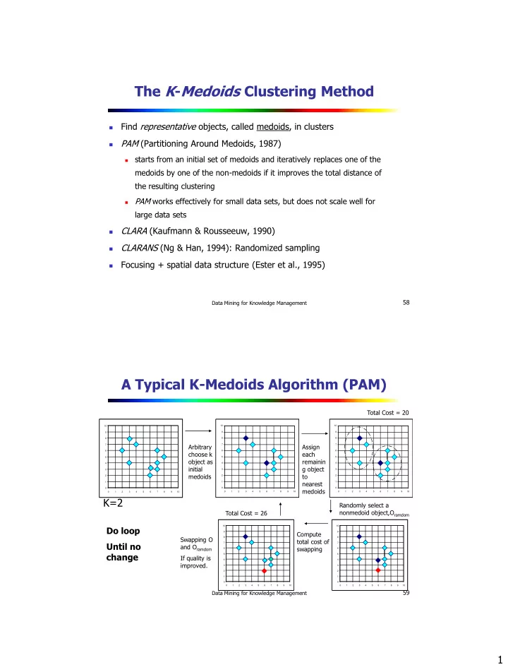A Typical K-Medoids Algorithm (PAM) Total Cost = 20 10 10 10 9 9 9 8 8 8 Arbitrary 7 Assign 7 7 6 6 6 choose k each 5 5 5 object as remainin 4 4 4 initial g object 3 3 3 medoids to 2 2 2 1 nearest 1 1 0 0 0 medoids 0 1 2 3 4 5 6 7 8 9 10 0 1 2 3 4 5 6 7 8 9 10 0 1 2 3 4 5 6 7 8 9 10 K=2 Randomly select a nonmedoid object,O ramdom Total Cost = 26 Do loop 10 10 9 Compute 9 Swapping O 8 8 total cost of Until no 7 7 and O ramdom swapping 6 6 change 5 5 If quality is 4 4 improved. 3 3 2 2 1 1 0 0 0 1 2 3 4 5 6 7 8 9 10 0 1 2 3 4 5 6 7 8 9 10 59 Data Mining for Knowledge Management 1

PAM (Partitioning Around Medoids) (1987)  PAM (Kaufman and Rousseeuw, 1987), built in Splus  Use real object to represent the cluster  Select k representative objects arbitrarily  For each pair of non-selected object h and selected object i , calculate the total swapping cost TC ih  For each pair of i and h ,  If TC ih < 0, i is replaced by h  Then assign each non-selected object to the most similar representative object  repeat steps 2-3 until there is no change 60 Data Mining for Knowledge Management What Is the Problem with PAM?  Pam is more robust than k-means in the presence of noise and outliers because a medoid is less influenced by outliers or other extreme values than a mean  Pam works efficiently for small data sets but does not scale well for large data sets.  O(k(n-k) 2 ) for each iteration where n is # of data,k is # of clusters  Sampling based method, CLARA(Clustering LARge Applications) 62 Data Mining for Knowledge Management 2

CLARA (Clustering Large Applications) (1990)  CLARA (Kaufmann and Rousseeuw in 1990)  Built in statistical analysis packages, such as S+  It draws multiple samples of the data set, applies PAM on each sample, and gives the best clustering as the output  Strength: deals with larger data sets than PAM  Weakness:  Efficiency depends on the sample size  A good clustering based on samples will not necessarily represent a good clustering of the whole data set if the sample is biased 63 Data Mining for Knowledge Management CLARANS (“Randomized” CLARA) (1994)  CLARANS (A Clustering Algorithm based on Randomized Search) (Ng and Han’94)  CLARANS draws sample of neighbors dynamically  The clustering process can be presented as searching a graph where every node is a potential solution, that is, a set of k medoids  If the local optimum is found, CLARANS starts with new randomly selected node in search for a new local optimum  It is more efficient and scalable than both PAM and CLARA  Focusing techniques and spatial access structures may further improve its performance (Ester et al.’95) 64 Data Mining for Knowledge Management 3

Roadmap 1. What is Cluster Analysis? 2. Types of Data in Cluster Analysis 3. A Categorization of Major Clustering Methods 4. Partitioning Methods 5. Hierarchical Methods 6. Density-Based Methods 7. Grid-Based Methods 8. Model-Based Methods 9. Clustering High-Dimensional Data 10. Constraint-Based Clustering 11. Summary 65 Data Mining for Knowledge Management Hierarchical Clustering  Use distance matrix as clustering criteria. This method does not require the number of clusters k as an input, but needs a termination condition Step 1 Step 2 Step 3 Step 4 Step 0 agglomerative (AGNES) a a b b a b c d e c c d e d d e e divisive Step 4 Step 3 Step 2 Step 1 Step 0 (DIANA) 66 Data Mining for Knowledge Management 4

AGNES (Agglomerative Nesting)  Introduced in Kaufmann and Rousseeuw (1990)  Implemented in statistical analysis packages, e.g., Splus  Use the Single-Link method and the dissimilarity matrix.  Merge nodes that have the least dissimilarity  Go on in a non-descending fashion  Eventually all nodes belong to the same cluster 10 10 10 9 9 9 8 8 8 7 7 7 6 6 6 5 5 5 4 4 4 3 3 3 2 2 2 1 1 1 0 0 0 0 1 2 3 4 5 6 7 8 9 10 0 1 2 3 4 5 6 7 8 9 10 0 1 2 3 4 5 6 7 8 9 10 67 Data Mining for Knowledge Management Dendrogram: Shows How the Clusters are Merged Decompose data objects into a several levels of nested partitioning (tree of clusters), called a dendrogram. A clustering of the data objects is obtained by cutting the dendrogram at the desired level, then each connected component forms a cluster. 68 Data Mining for Knowledge Management 5

DIANA (Divisive Analysis)  Introduced in Kaufmann and Rousseeuw (1990)  Implemented in statistical analysis packages, e.g., Splus  Inverse order of AGNES  Eventually each node forms a cluster on its own 10 10 10 9 9 9 8 8 8 7 7 7 6 6 6 5 5 5 4 4 4 3 3 3 2 2 2 1 1 1 0 0 0 0 1 2 3 4 5 6 7 8 9 10 0 1 2 3 4 5 6 7 8 9 10 0 1 2 3 4 5 6 7 8 9 10 69 Data Mining for Knowledge Management Recent Hierarchical Clustering Methods  Major weakness of agglomerative clustering methods  do not scale well: time complexity of at least O ( n 2 ), where n is the number of total objects  can never undo what was done previously  Integration of hierarchical with distance-based clustering  BIRCH (1996): uses CF-tree and incrementally adjusts the quality of sub-clusters  ROCK (1999): clustering categorical data by neighbor and link analysis  CHAMELEON (1999): hierarchical clustering using dynamic modeling 70 Data Mining for Knowledge Management 6

BIRCH (1996)  Birch: Balanced Iterative Reducing and Clustering using Hierarchies (Zhang, Ramakrishnan & Livny, SIGMOD ’ 96)  Incrementally construct a CF (Clustering Feature) tree, a hierarchical data structure for multiphase clustering  Phase 1: scan DB to build an initial in-memory CF tree (a multi-level compression of the data that tries to preserve the inherent clustering structure of the data)  Phase 2: use an arbitrary clustering algorithm to cluster the leaf nodes of the CF-tree  Scales linearly : finds a good clustering with a single scan and improves the quality with a few additional scans  Weakness: handles only numeric data, and sensitive to the order of the data record. 71 Data Mining for Knowledge Management Clustering Feature Vector in BIRCH Clustering Feature: CF = (N, LS, SS) N : Number of data points LS:  N i=1 =X i SS:  N 2 i=1 =X i CF = (5, (16,30),(54,190)) (3,4) 10 9 8 (2,6) 7 6 (4,5) 5 4 3 (4,7) 2 1 0 (3,8) 0 1 2 3 4 5 6 7 8 9 10 72 Data Mining for Knowledge Management 7

CF-Tree in BIRCH Clustering feature:  summary of the statistics for a given subcluster: the 0-th, 1st and 2nd  moments of the subcluster from the statistical point of view. registers crucial measurements for computing cluster and utilizes storage  efficiently A CF tree is a height-balanced tree that stores the clustering features for a hierarchical clustering A nonleaf node in a tree has descendants or “children”  The nonleaf nodes store sums of the CFs of their children  A CF tree has two parameters  Branching factor: specify the maximum number of children.  threshold: max diameter of sub-clusters stored at the leaf nodes  73 Data Mining for Knowledge Management The CF Tree Structure Root CF 1 CF 2 CF 3 CF 6 B = 7 child 1 child 2 child 3 child 6 L = 6 Non-leaf node CF 1 CF 2 CF 3 CF 5 child 1 child 2 child 3 child 5 Leaf node Leaf node prev CF 1 CF 2 CF 6 next prev CF 1 CF 2 CF 4 next 74 Data Mining for Knowledge Management 8

Clustering Categorical Data: The ROCK Algorithm ROCK: RObust Clustering using linKs  S. Guha, R. Rastogi & K. Shim, ICDE’99  Major ideas  Not distance-based  Use links to measure similarity/proximity  Measure similarity between points, as well as between their corresponding  neighborhoods  two points are closer together if they share some of their neighbors Algorithm: sampling-based clustering  Draw random sample  Cluster with links  Label data in disk  Computational complexity: O n   2 2 ( nm m n log ) n  m a 75 Data Mining for Knowledge Management Similarity Measure in ROCK Traditional measures for categorical data may not work well, e.g.,  Jaccard coefficient Example: Two groups (clusters) of transactions  C 1 . <a, b, c, d, e>: {a, b, c}, {a, b, d}, {a, b, e}, {a, c, d}, {a, c, e},  {a, d, e}, {b, c, d}, {b, c, e}, {b, d, e}, {c, d, e} C 2 . <a, b, f, g>: {a, b, f}, {a, b, g}, {a, f, g}, {b, f, g}  76 Data Mining for Knowledge Management 9