The DSM data matrix DSM data are given as a term-term or term-context - - PowerPoint PPT Presentation

Introduction The DSM matrix

The DSM data matrix

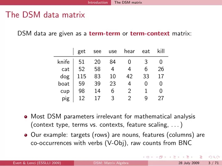
DSM data are given as a term-term or term-context matrix:

get see use hear eat kill knife 51 20 84 3 cat 52 58 4 4 6 26 dog 115 83 10 42 33 17 boat 59 39 23 4 cup 98 14 6 2 1 pig 12 17 3 2 9 27

Most DSM parameters irrelevant for mathematical analysis (context type, terms vs. contexts, feature scaling, . . . ) Our example: targets (rows) are nouns, features (columns) are co-occurrences with verbs (V-Obj), raw counts from BNC

Evert & Lenci (ESSLLI 2009) DSM: Matrix Algebra 28 July 2009 3 / 71

Introduction The DSM matrix

The DSM data matrix

DSM data are given as a term-term or term-context matrix: M =         51 20 84 3 52 58 4 4 6 26 115 83 10 42 33 17 59 39 23 4 98 14 6 2 1 12 17 3 2 9 27         Mathematical notation: matrix M of real numbers Each row is a feature vector for one of the target terms, e.g. vcat =

• 52

58 4 4 6 26

• n-dimensional vector space Rn ∋ v = (v1, . . . , vn)

Evert & Lenci (ESSLLI 2009) DSM: Matrix Algebra 28 July 2009 4 / 71

Introduction Geometric interpretation

Why vector spaces?

Vector spaces encode basic geometric intuitions

☞ geometric interpretation of numerical feature lists ☞ one reason why linear algebra is such a useful tool

Evert & Lenci (ESSLLI 2009) DSM: Matrix Algebra 28 July 2009 5 / 71

Introduction Geometric interpretation

Why vector spaces?

Vector spaces encode basic geometric intuitions

☞ geometric interpretation of numerical feature lists ☞ one reason why linear algebra is such a useful tool

Interpretation of vectors x, y, . . . ∈ Rn as points in n-dimensional Euclidean (= intuitive) space

◮ n = 2 ➜ Euclidean plane ◮ n = 3 ➜ three-dimensional Euclidean space Evert & Lenci (ESSLLI 2009) DSM: Matrix Algebra 28 July 2009 5 / 71

Introduction Geometric interpretation

Why vector spaces?

Vector spaces encode basic geometric intuitions

☞ geometric interpretation of numerical feature lists ☞ one reason why linear algebra is such a useful tool

Interpretation of vectors x, y, . . . ∈ Rn as points in n-dimensional Euclidean (= intuitive) space

◮ n = 2 ➜ Euclidean plane ◮ n = 3 ➜ three-dimensional Euclidean space

Exploit geometric intuition for analysis of DSM data as group of points or arrows in Euclidean space

◮ distance, length, direction, angle, dimension, . . . ◮ intuitive in R2 and R3 ◮ can be generalised to higher dimensions

☞ I may refer to feature vectors for target terms as “data points”

Evert & Lenci (ESSLLI 2009) DSM: Matrix Algebra 28 July 2009 5 / 71

Introduction Geometric interpretation

The geometric interpretation of vectors

Vectors as points

Vectors like u = (4, 2) and v = (3, 5) can be understood as the coordinates of points in the Euclidean plane In this interpretation, vectors identify specific locations in the plane

x1

u = (4, 2)

x2

1 2 3 4 5 1 2 3 4 5 6 6

v = (3, 5)

Evert & Lenci (ESSLLI 2009) DSM: Matrix Algebra 28 July 2009 6 / 71

Introduction Geometric interpretation

The geometric interpretation of vectors

Vectors as arrows & vector addition

Vectors can also be interpreted as “displacement arrows” between points Arrow from u to v is de- scribed by vector (−1, 3) Calculated as pointwise difference between components of v and u: v −u = (v1 −u1, v2 −u2) General operation: vector addition

x1

u = (4, 2)

x2

1 2 3 4 5 1 2 3 4 5 6 6

v = (3, 5) v-u = (-1, 3)

Evert & Lenci (ESSLLI 2009) DSM: Matrix Algebra 28 July 2009 7 / 71

Introduction Geometric interpretation

The geometric interpretation of vectors

Vectors as arrows

Vectors as arrows are position-independent y − x = v − u if the relative positions of x and y are the same as those of u and v Regardless of their location in the plane

x1

x = (6, 3.5)

x2

1 2 3 4 5 1 2 3 4 5 6 6

y = (4, 6.5) y-x = v-u = (-1, 3)

Evert & Lenci (ESSLLI 2009) DSM: Matrix Algebra 28 July 2009 8 / 71

Introduction Geometric interpretation

The geometric interpretation of vectors

Direction & scalar multiplication

Intuitively, arrows have a length and direction Arrows point in the same direction iff they are multiples of each other: scalar multiplication λu = (λu1, λu2) with constant factor λ ∈ R For λ < 0, arrows have

• pposite directions

−u = (−1) · u is the inverse arrow of u

x1 x2

1 2 3 4 5 1 2 3 4 5 6 6

u 2u

• u

Evert & Lenci (ESSLLI 2009) DSM: Matrix Algebra 28 July 2009 9 / 71

Introduction Geometric interpretation

The geometric interpretation of vectors

Linking points and arrows

Points in the plane can be identified by displace- ment arrows from fixed reference point A natural reference point is the origin 0 = (0, 0) These arrows are given by the same vectors as the point coordinates

x1

• rigin

(0,0) (4, 2)

x2

1 2 3 4 5 1 2 3 4 5 6 6

(3, 5)

Evert & Lenci (ESSLLI 2009) DSM: Matrix Algebra 28 July 2009 10 / 71

Introduction Geometric interpretation

Geometric interpretation of DSM data matrix

Reduce DSM matrix to two dimensions for visualisation: get use knife 51 84 cat 52 4 dog 115 10 boat 59 23 cup 98 6 pig 12 3

Evert & Lenci (ESSLLI 2009) DSM: Matrix Algebra 28 July 2009 11 / 71

Introduction Geometric interpretation

Geometric interpretation of DSM data matrix

Reduce DSM matrix to two dimensions for visualisation: get use knife 51 84 cat 52 4 dog 115 10 boat 59 23 cup 98 6 pig 12 3

• 20

40 60 80 100 120 20 40 60 80 100 120

Two dimensions of English V−Obj DSM

get use

cat dog knife boat

Evert & Lenci (ESSLLI 2009) DSM: Matrix Algebra 28 July 2009 11 / 71

Vector spaces Formal definition

The n-dimensional Euclidean space

The mathematical basis for matrix algebra is the theory of vector spaces, also known as linear algebra Before we focue on the analsis of DSM matrices, we will look at some fundamental definitions and results of linear algebra

Evert & Lenci (ESSLLI 2009) DSM: Matrix Algebra 28 July 2009 12 / 71

Vector spaces Formal definition

The n-dimensional Euclidean space

The mathematical basis for matrix algebra is the theory of vector spaces, also known as linear algebra Before we focue on the analsis of DSM matrices, we will look at some fundamental definitions and results of linear algebra Definition: the n-dimensional real Euclidean vector space Rn is the set of all real-valued vectors x = (x1, . . . , xn) of length n, with the following operations:

◮ vector addition: u + v := (u1 + v1, . . . , un + vn) ◮ scalar multiplication: λu := (λu1, . . . , λun) for λ ∈ R Evert & Lenci (ESSLLI 2009) DSM: Matrix Algebra 28 July 2009 12 / 71

Vector spaces Formal definition

The n-dimensional Euclidean space

Important properties of the addition and s-multiplication

• perations in Rn
• 1. (u + v) + w = u + (v + w)
• 2. u + 0 = 0 + u = u
• 3. ∀u ∃(−u) : u + (−u) = (−u) + u = 0
• 4. u + v = v + u
• 5. (λ + µ)u = λu + µu
• 6. (λµ)u = λ(µu)
• 7. 1 · u = u
• 8. λ(u + v) = λu + λv

for any u, v, w ∈ Rn and λ, µ ∈ R

Evert & Lenci (ESSLLI 2009) DSM: Matrix Algebra 28 July 2009 13 / 71

Vector spaces Formal definition

The axioms of a general vector space

Abstract vector space over the real numbers R = set V of vectors u ∈ V with operations

◮ u + v ∈ V for u, v ∈ V (addition) ◮ λu ∈ V for λ ∈ R, u ∈ V (scalar multiplication)

Addition and s-multiplication must satisfy the axioms

• 1. (u + v) + w = u + (v + w)
• 2. u + 0 = 0 + u = u
• 3. ∀u ∃u′ : u + u′ = u′ + u = 0
• 4. u + v = v + u
• 5. (λ + µ)u = λu + µu
• 6. (λµ)u = λ(µu)
• 7. 1 · u = u
• 8. λ(u + v) = λu + λv

for any u, v, w ∈ V and λ, µ ∈ R 0 is the unique neutral element of V , and the unique inverse u′ of u is often written as −u

Evert & Lenci (ESSLLI 2009) DSM: Matrix Algebra 28 July 2009 14 / 71

Vector spaces Formal definition

Further properties of vector spaces

Further properties of vector spaces:

◮ 0 · u = 0 ◮ λ0 = 0 ◮ λu = 0 ⇒ λ = 0 ∨ u = 0 ◮ (−λ)u = λ(−u) = −(λu) =: −λu Evert & Lenci (ESSLLI 2009) DSM: Matrix Algebra 28 July 2009 15 / 71

Vector spaces Formal definition

Further properties of vector spaces

Further properties of vector spaces:

◮ 0 · u = 0 ◮ λ0 = 0 ◮ λu = 0 ⇒ λ = 0 ∨ u = 0 ◮ (−λ)u = λ(−u) = −(λu) =: −λu

It is easy to show these properties for Rn, but they also follow directly from the general axioms for all vector spaces

Evert & Lenci (ESSLLI 2009) DSM: Matrix Algebra 28 July 2009 15 / 71

Vector spaces Formal definition

Further properties of vector spaces

Further properties of vector spaces:

◮ 0 · u = 0 ◮ λ0 = 0 ◮ λu = 0 ⇒ λ = 0 ∨ u = 0 ◮ (−λ)u = λ(−u) = −(λu) =: −λu

It is easy to show these properties for Rn, but they also follow directly from the general axioms for all vector spaces A non-trivial example: vector space C[a, b] of continuous real functions f : x → f (x) over the interval [a, b]

◮ vector addition: ∀f , g ∈ C[a, b],

we define f + g by (f + g)(x) := f (x) + g(x)

◮ s-multiplication: ∀λ ∈ R and ∀f ∈ C[a, b],

we define λf by (λf )(x) := λ · f (x)

☞ One can show that C[a, b] satisfies the vector space axioms

Evert & Lenci (ESSLLI 2009) DSM: Matrix Algebra 28 July 2009 15 / 71

Vector spaces Basis & linear subspace

Linear combinations & dimensionality

Linear combination of vectors u(1), . . . , u(n): λ1u(1) + λ2u(2) + · · · + λnu(n) for any coefficients λ1, . . . , λn ∈ R

◮ intuition: all vectors that can be constructed from

u(1), . . . , u(n) using the basic vector operations

Evert & Lenci (ESSLLI 2009) DSM: Matrix Algebra 28 July 2009 16 / 71

Vector spaces Basis & linear subspace

Linear combinations & dimensionality

Linear combination of vectors u(1), . . . , u(n): λ1u(1) + λ2u(2) + · · · + λnu(n) for any coefficients λ1, . . . , λn ∈ R

◮ intuition: all vectors that can be constructed from

u(1), . . . , u(n) using the basic vector operations

u(1), . . . , u(n) are linearly independent iff λ1u(1) + λ2u(2) + · · · + λnu(n) = 0 implies λ1 = λ2 = · · · = λn = 0

Evert & Lenci (ESSLLI 2009) DSM: Matrix Algebra 28 July 2009 16 / 71

Vector spaces Basis & linear subspace

Linear combinations & dimensionality

Linear combination of vectors u(1), . . . , u(n): λ1u(1) + λ2u(2) + · · · + λnu(n) for any coefficients λ1, . . . , λn ∈ R

◮ intuition: all vectors that can be constructed from

u(1), . . . , u(n) using the basic vector operations

u(1), . . . , u(n) are linearly independent iff λ1u(1) + λ2u(2) + · · · + λnu(n) = 0 implies λ1 = λ2 = · · · = λn = 0 Otherwise, they are linearly dependent

◮ equivalent: one u(i) is a linear combination of the other vectors Evert & Lenci (ESSLLI 2009) DSM: Matrix Algebra 28 July 2009 16 / 71

Vector spaces Basis & linear subspace

Linear combinations & dimensionality

Largest n ∈ N for which there is a set of n linearly independent vectors u(i) ∈ V is called the dimension of V : dim V = n It can be shown that dim Rn = n

Evert & Lenci (ESSLLI 2009) DSM: Matrix Algebra 28 July 2009 17 / 71

Vector spaces Basis & linear subspace

Linear combinations & dimensionality

Largest n ∈ N for which there is a set of n linearly independent vectors u(i) ∈ V is called the dimension of V : dim V = n It can be shown that dim Rn = n If there is no maximal number of linearly independent vectors, the vector space is infinite-dimensional (dim V = ∞) An example is dim C[a, b] = ∞ (easy to show)

Evert & Lenci (ESSLLI 2009) DSM: Matrix Algebra 28 July 2009 17 / 71

Vector spaces Basis & linear subspace

Linear combinations & dimensionality

Largest n ∈ N for which there is a set of n linearly independent vectors u(i) ∈ V is called the dimension of V : dim V = n It can be shown that dim Rn = n If there is no maximal number of linearly independent vectors, the vector space is infinite-dimensional (dim V = ∞) An example is dim C[a, b] = ∞ (easy to show) Every finite-dimensional vector space V is isomorphic to the Euclidean space Rn (with n = dim V )

☞ We will be able to prove this in a little while

Evert & Lenci (ESSLLI 2009) DSM: Matrix Algebra 28 July 2009 17 / 71

Vector spaces Basis & linear subspace

Basis & coordinates

A set of vectors b(1), . . . , b(n) ∈ V is called a basis of V iff every u ∈ V can be written as a linear combination u = x1b(1) + x2b(2) + · · · + xnb(n) with unique coefficients x1, . . . , xn Number of vectors in a basis = dim V

Evert & Lenci (ESSLLI 2009) DSM: Matrix Algebra 28 July 2009 18 / 71

Vector spaces Basis & linear subspace

Basis & coordinates

A set of vectors b(1), . . . , b(n) ∈ V is called a basis of V iff every u ∈ V can be written as a linear combination u = x1b(1) + x2b(2) + · · · + xnb(n) with unique coefficients x1, . . . , xn Number of vectors in a basis = dim V For every n-dimensional vector space V , a set of n vectors b(1), . . . , b(n) ∈ V is a basis iff they are linearly independent

☞ Can you think of a proof?

Evert & Lenci (ESSLLI 2009) DSM: Matrix Algebra 28 July 2009 18 / 71

Vector spaces Basis & linear subspace

Basis & coordinates

The unique coefficients x1, . . . , xn are called the coordinates

• f u wrt. the basis B :=
• b(1), . . . , b(n)

: u ≡B      x1 x2 . . . xn      =: x

Evert & Lenci (ESSLLI 2009) DSM: Matrix Algebra 28 July 2009 19 / 71

Vector spaces Basis & linear subspace

Basis & coordinates

The unique coefficients x1, . . . , xn are called the coordinates

• f u wrt. the basis B :=
• b(1), . . . , b(n)

: u ≡B      x1 x2 . . . xn      =: x x ∈ Rn is the coordinate vector of u ∈ V wrt. B

☞ V is isomorphic to Rn by virtue of this correspondence

Evert & Lenci (ESSLLI 2009) DSM: Matrix Algebra 28 July 2009 19 / 71

Vector spaces Basis & linear subspace

Basis & coordinates

The unique coefficients x1, . . . , xn are called the coordinates

• f u wrt. the basis B :=
• b(1), . . . , b(n)

: u ≡B      x1 x2 . . . xn      =: x x ∈ Rn is the coordinate vector of u ∈ V wrt. B

☞ V is isomorphic to Rn by virtue of this correspondence

We can think of the rows (or columns) of a DSM matrix M as coordinates in an abstract vector space

◮ coordinate transformations play an important role for DSMs Evert & Lenci (ESSLLI 2009) DSM: Matrix Algebra 28 July 2009 19 / 71

Vector spaces Basis & linear subspace

Basis & coordinates

The components (u1, u2, . . . , un) of a number vector u ∈ Rn correspond to its natural coordinates u = (u1, u2, . . . , un) ≡E      u1 u2 . . . un      according to the standard basis e(1), . . . , e(n) of Rn: e(1) = (1, 0, . . . , 0) e(2) = (0, 1, . . . , 0) . . . e(n) = (0, 0, . . . , 1)

Evert & Lenci (ESSLLI 2009) DSM: Matrix Algebra 28 July 2009 20 / 71

Vector spaces Basis & linear subspace

Basis & coordinates

u = (4, 5) ∈ R2 Basis B of R2: b(1) = (2, 1) b(2) = (−1, 1) u ≡B 3 2

• x1

x2

1 2 3 4 5 1 2 3 4 5 6 6

u=(4,5) b(2) b(1)

Evert & Lenci (ESSLLI 2009) DSM: Matrix Algebra 28 July 2009 21 / 71

Vector spaces Basis & linear subspace

Basis & coordinates

u = (4, 5) ∈ R2 Basis B of R2: b(1) = (2, 1) b(2) = (−1, 1) u ≡B 3 2

• Standard basis:

e(1) = (1, 0) e(2) = (0, 1) u ≡E 4 5

• x1

x2

1 2 3 4 5 1 2 3 4 5 6 6

u=(4,5) b(2) b(1) e(1) e(2)

Evert & Lenci (ESSLLI 2009) DSM: Matrix Algebra 28 July 2009 21 / 71

Vector spaces Basis & linear subspace

Linear subspaces

The set of all linear combinations of vectors b(1), . . . , b(k) ∈ V is called the span sp

• b(1), . . . , b(k)

:=

• λ1b(1) + · · · + λkb(k) | λi ∈ R
• Evert & Lenci (ESSLLI 2009)

DSM: Matrix Algebra 28 July 2009 22 / 71

Vector spaces Basis & linear subspace

Linear subspaces

The set of all linear combinations of vectors b(1), . . . , b(k) ∈ V is called the span sp

• b(1), . . . , b(k)

:=

• λ1b(1) + · · · + λkb(k) | λi ∈ R
• sp
• b(1), . . . , b(k)

forms a linear subspace of V

◮ a linear subspace is a subset of V that is closed under vector

addition and scalar multiplication

Evert & Lenci (ESSLLI 2009) DSM: Matrix Algebra 28 July 2009 22 / 71

Vector spaces Basis & linear subspace

Linear subspaces

The set of all linear combinations of vectors b(1), . . . , b(k) ∈ V is called the span sp

• b(1), . . . , b(k)

:=

• λ1b(1) + · · · + λkb(k) | λi ∈ R
• sp
• b(1), . . . , b(k)

forms a linear subspace of V

◮ a linear subspace is a subset of V that is closed under vector

addition and scalar multiplication

b(1), . . . , b(k) form a basis of sp

• b(1), . . . , b(k)

iff they are linearly independent ☞ Can you prove that every linear subspace of Rn has a basis?

Evert & Lenci (ESSLLI 2009) DSM: Matrix Algebra 28 July 2009 22 / 71

Vector spaces Basis & linear subspace

Linear subspaces

The set of all linear combinations of vectors b(1), . . . , b(k) ∈ V is called the span sp

• b(1), . . . , b(k)

:=

• λ1b(1) + · · · + λkb(k) | λi ∈ R
• sp
• b(1), . . . , b(k)

forms a linear subspace of V

◮ a linear subspace is a subset of V that is closed under vector

addition and scalar multiplication

b(1), . . . , b(k) form a basis of sp

• b(1), . . . , b(k)

iff they are linearly independent ☞ Can you prove that every linear subspace of Rn has a basis? The rank of vectors b(1), . . . , b(k) is the dimension of their span, corresponding to the largest number of linearly independent vectors among them

Evert & Lenci (ESSLLI 2009) DSM: Matrix Algebra 28 July 2009 22 / 71

Vector spaces Basis & linear subspace

Linear combinations & linear subspace

Example: linear subspace U ⊆ R3 spanned by vectors b(1) = (6, 0, 2), b(2) = (0, 3, 3) and b(3) = (3, 1, 2)

◮ dim U = 2 (why?)

x1 x3

1 2 3 4 5 1 2 3 4 5 6 6

x2

Evert & Lenci (ESSLLI 2009) DSM: Matrix Algebra 28 July 2009 23 / 71

Vector spaces Basis & linear subspace

Linear combinations & linear subspace

Example: linear subspace U ⊆ R3 spanned by vectors b(1) = (6, 0, 2), b(2) = (0, 3, 3) and b(3) = (3, 1, 2)

◮ dim U = 2 (because b(2) = 3b(3) − 3

2b(1)) x1 x3

1 2 3 4 5 1 2 3 4 5 6 6

x2

Evert & Lenci (ESSLLI 2009) DSM: Matrix Algebra 28 July 2009 23 / 71

Matrix algebra in a nutshell

Matrix as list of vectors

Vector u ∈ Rn = list of real numbers (coordinates)

Evert & Lenci (ESSLLI 2009) DSM: Matrix Algebra 28 July 2009 24 / 71

Matrix algebra in a nutshell

Matrix as list of vectors

Vector u ∈ Rn = list of real numbers (coordinates) List of k vectors = rectangular array of real numbers, called a n × k matrix (or k × n row matrix)

Evert & Lenci (ESSLLI 2009) DSM: Matrix Algebra 28 July 2009 24 / 71

Matrix algebra in a nutshell

Matrix as list of vectors

Vector u ∈ Rn = list of real numbers (coordinates) List of k vectors = rectangular array of real numbers, called a n × k matrix (or k × n row matrix) Example: vectors u, v ∈ R3 u ≡   3 2   , v ≡   2 2 1   form the columns of a matrix A: A =     . . . . . . u v . . . . . .     =   3 2 2 2 1   =   a11 a12 a21 a22 a31 a32  

Evert & Lenci (ESSLLI 2009) DSM: Matrix Algebra 28 July 2009 24 / 71

Matrix algebra in a nutshell

Matrix = list of vectors

rank (A) = rank of the list of column vectors Column matrices are a convention in linear algebra But DSM matrix often has row vectors for the target terms

Evert & Lenci (ESSLLI 2009) DSM: Matrix Algebra 28 July 2009 25 / 71

Matrix algebra in a nutshell

Matrix = list of vectors

rank (A) = rank of the list of column vectors Column matrices are a convention in linear algebra But DSM matrix often has row vectors for the target terms Row rank and column rank of a matrix A are always the same (this is not trivial!)

Evert & Lenci (ESSLLI 2009) DSM: Matrix Algebra 28 July 2009 25 / 71

Matrix algebra in a nutshell

Matrices and linear equation systems

Matrices are a versatile instrument and a convenient way to express linear operations on sets of numbers E.g. coefficient matrix of a linear system of equations: a11x1 + a12x2 + · · · + a1nxn = b1 a21x1 + a22x2 + · · · + a2nxn = b2 . . . ak1x1 + ak2x2 + · · · + aknxn = bk

Evert & Lenci (ESSLLI 2009) DSM: Matrix Algebra 28 July 2009 26 / 71

Matrix algebra in a nutshell

Matrices and linear equation systems

Matrices are a versatile instrument and a convenient way to express linear operations on sets of numbers E.g. coefficient matrix of a linear system of equations: a11x1 + a12x2 + · · · + a1nxn = b1 a21x1 + a22x2 + · · · + a2nxn = b2 . . . ak1x1 + ak2x2 + · · · + aknxn = bk ➥ A =    a11 · · · a1n . . . . . . ak1 · · · akn    , x =      x1 x2 . . . xn      , b =    b1 . . . bk   

Evert & Lenci (ESSLLI 2009) DSM: Matrix Algebra 28 July 2009 26 / 71

Matrix algebra in a nutshell

Matrix algebra

Concise notation of linear equation system by appropriate definition of matrix-vector multiplication a11x1 + a12x2 + · · · + a1nxn = b1 a21x1 + a22x2 + · · · + a2nxn = b2 . . . ak1x1 + ak2x2 + · · · + aknxn = bk ➥    a11 · · · a1n . . . . . . ak1 · · · akn    ·      x1 x2 . . . xn      =    b1 . . . bk   

Evert & Lenci (ESSLLI 2009) DSM: Matrix Algebra 28 July 2009 27 / 71

Matrix algebra in a nutshell

Matrix algebra

Concise notation of linear equation system by appropriate definition of matrix-vector multiplication a11x1 + a12x2 + · · · + a1nxn = b1 a21x1 + a22x2 + · · · + a2nxn = b2 . . . ak1x1 + ak2x2 + · · · + aknxn = bk ➥    a11 · · · a1n . . . . . . ak1 · · · akn    ·      x1 x2 . . . xn      =    b1 . . . bk    ➥ A · x = b

Evert & Lenci (ESSLLI 2009) DSM: Matrix Algebra 28 July 2009 27 / 71

Matrix algebra in a nutshell

Matrix algebra

The set of all real-valued k × n matrices forms a (k · n)-dimensional vector space over R:

◮ A + B is defined by element-wise addition ◮ λA is defined by element-wise s-multiplication ◮ these operations satisfy all vector space axioms Evert & Lenci (ESSLLI 2009) DSM: Matrix Algebra 28 July 2009 28 / 71

Matrix algebra in a nutshell

Matrix algebra

The set of all real-valued k × n matrices forms a (k · n)-dimensional vector space over R:

◮ A + B is defined by element-wise addition ◮ λA is defined by element-wise s-multiplication ◮ these operations satisfy all vector space axioms

Additional operation: matrix multiplication

◮ two equation systems: z = B · y and y = C · x ◮ by inserting the expressions for y into the first system,

we can express z directly in terms of x (and use this e.g. to solve the equations for x)

◮ the result is a linear equation system z = A · x

☞ define matrix multiplication such that A = B · C

Evert & Lenci (ESSLLI 2009) DSM: Matrix Algebra 28 July 2009 28 / 71

Matrix algebra in a nutshell

Matrix multiplication

  aij   =   bi1 · · · bin   ·       c1j . . . . . . cnj       A = B · C (k × m) (k × n) (n × m) B and C must be conformable

Evert & Lenci (ESSLLI 2009) DSM: Matrix Algebra 28 July 2009 29 / 71

Matrix algebra in a nutshell

Matrix multiplication

  aij   =   bi1 · · · bin   ·       c1j . . . . . . cnj       A = B · C (k × m) (k × n) (n × m) B and C must be conformable

Evert & Lenci (ESSLLI 2009) DSM: Matrix Algebra 28 July 2009 29 / 71

Matrix algebra in a nutshell

Matrix multiplication

 aij   =  bi1 · · · bin   ·       c1j . . . . . . cnj       A = B · C (k × m) (k × n) (n × m) B and C must be conformable

Evert & Lenci (ESSLLI 2009) DSM: Matrix Algebra 28 July 2009 30 / 71

Matrix algebra in a nutshell

Matrix multiplication

 aij   =  bi1 · · · bin   ·       c1j . . . . . . cnj       A = B · C (k × m) (k × n) (n × m) B and C must be conformable ☞ A · x corresponds to matrix multiplication of A with a single-column matrix (containing the vector x)

◮ convention: vector = column matrix Evert & Lenci (ESSLLI 2009) DSM: Matrix Algebra 28 July 2009 30 / 71

Matrix algebra in a nutshell

Matrix multiplication

Algebra = vector space + multiplication operation with the following properties:

◮ A(BC) = (AB)C =: ABC ◮ A(B + B′) = AB + AB′ ◮ (A + A′)B = AB + A′B ◮ (λA)B = A(λB) = λ(AB) =: λAB ◮ A · 0 = 0,

0 · B = 0

◮ A · I = A,

I · B = B

where A, B and C are conformable matrices 0 is a zero matrix of arbitrary dimensions I is a square identity matrix of arbitrary dimensions: I :=    1 ... 1   

Evert & Lenci (ESSLLI 2009) DSM: Matrix Algebra 28 July 2009 31 / 71

Matrix algebra in a nutshell

Transposition

The transpose AT of a matrix A swaps rows and columns:   a1 b1 a2 b2 a3 b3  

T

= a1 a2 a3 b1 b2 b3

• Evert & Lenci (ESSLLI 2009)

DSM: Matrix Algebra 28 July 2009 32 / 71

Matrix algebra in a nutshell

Transposition

The transpose AT of a matrix A swaps rows and columns:   a1 b1 a2 b2 a3 b3  

T

= a1 a2 a3 b1 b2 b3

• Properties of the transpose:

◮ (A + B)T = AT + BT ◮ (λA)T = λ(AT) =: λAT ◮ (A · B)T = BT · AT

[note the different order of A and B!]

◮ rank

• AT

= rank (A)

◮ IT = I Evert & Lenci (ESSLLI 2009) DSM: Matrix Algebra 28 July 2009 32 / 71

Matrix algebra in a nutshell

Transposition

The transpose AT of a matrix A swaps rows and columns:   a1 b1 a2 b2 a3 b3  

T

= a1 a2 a3 b1 b2 b3

• Properties of the transpose:

◮ (A + B)T = AT + BT ◮ (λA)T = λ(AT) =: λAT ◮ (A · B)T = BT · AT

[note the different order of A and B!]

◮ rank

• AT

= rank (A)

◮ IT = I

A is called symmetric iff AT = A

◮ symmetric matrices have many special properties that will

become important later (e.g. eigenvalues)

Evert & Lenci (ESSLLI 2009) DSM: Matrix Algebra 28 July 2009 32 / 71

Matrix algebra in a nutshell

Vectors and matrices

A coordinate vector x ∈ Rn can be identified with a n × 1 matrix (i.e. a single-column matrix): x =    x1 . . . xn    =

• x1

· · · xn T

Evert & Lenci (ESSLLI 2009) DSM: Matrix Algebra 28 July 2009 33 / 71

Matrix algebra in a nutshell

Vectors and matrices

A coordinate vector x ∈ Rn can be identified with a n × 1 matrix (i.e. a single-column matrix): x =    x1 . . . xn    =

• x1

· · · xn T Multiplication of a matrix A containing the vectors a(1), . . . , a(k) with a vector of coefficients λ1, . . . , λk yields a linear combination of a(1), . . . , a(k): A ·    λ1 . . . λk    = λ1a(1) + · · · + λka(k)

Evert & Lenci (ESSLLI 2009) DSM: Matrix Algebra 28 July 2009 33 / 71

Matrix algebra with R

R as a toy DSM laboratory

Matrix algebra is a powerful and convenient tool in numerical mathematics ➜ implement DSM with matrix operations Specialised (and highly optimised) libraries are available for various programming languages (C, C++, Perl, Python, . . . ) Some numerical programming environments are even based entirely on matrix algebra (Matlab, Octave, NumPy/Sage) Statistical software packages like R also support matrices

Evert & Lenci (ESSLLI 2009) DSM: Matrix Algebra 28 July 2009 34 / 71

Matrix algebra with R

R as a toy DSM laboratory

Matrix algebra is a powerful and convenient tool in numerical mathematics ➜ implement DSM with matrix operations Specialised (and highly optimised) libraries are available for various programming languages (C, C++, Perl, Python, . . . ) Some numerical programming environments are even based entirely on matrix algebra (Matlab, Octave, NumPy/Sage) Statistical software packages like R also support matrices R as a DSM laboratory for toy models http://www.r-project.org/ Integrates efficient matrix operations with statistical analysis, clustering, machine learning, visualisation, . . .

Evert & Lenci (ESSLLI 2009) DSM: Matrix Algebra 28 July 2009 34 / 71

Matrix algebra with R

Matrix algebra with R

Vectors in R: u1 <- c(3, 0, 2) u2 <- c(0, 2, 2) v <- 1:6 print(v)

[1] 1 2 3 4 5 6

Defining matrices: A <- matrix(v, nrow=3) print(A)

[,1] [,2] [1,] 1 4 [2,] 2 5 [3,] 3 6

Evert & Lenci (ESSLLI 2009) DSM: Matrix Algebra 28 July 2009 35 / 71

Matrix algebra with R

Matrix algebra in R

Matrix of column vectors: B <- cbind(u1, u2) print(B)

u1 u2 [1,] 3 [2,] 2 [3,] 2 2

Matrix of row vectors: C <- rbind(u1, u2) print(C)

[,1] [,2] [,3] u1 3 2 u2 2 2

Evert & Lenci (ESSLLI 2009) DSM: Matrix Algebra 28 July 2009 36 / 71

Matrix algebra with R

Matrix algebra in R

Matrix multiplication: A %*% C

[,1] [,2] [,3] [1,] 3 8 10 [2,] 6 10 14 [3,] 9 12 18

NB: * does not perform matrix multiplication Also for multiplication of matrix with vector: C %*% c(1,1,0)

[,1] u1 3 u2 2

☞ result of multiplication is a column vector (i.e. plain vectors are interpreted as column vectors in matrix operations)

Evert & Lenci (ESSLLI 2009) DSM: Matrix Algebra 28 July 2009 37 / 71

Matrix algebra with R

Matrix algebra in R

Transpose of matrix: t(A)

[,1] [,2] [,3] [1,] 1 2 3 [2,] 4 5 6

Transposition of vectors: t(u1) (row vector)

[,1] [,2] [,3] [1,] 3 2

t(t(u1)) (explicit column vector)

[,1] [1,] 3 [2,] [3,] 2

Evert & Lenci (ESSLLI 2009) DSM: Matrix Algebra 28 July 2009 38 / 71

Matrix algebra with R

Matrix algebra in R

Rank of a matrix: qr(A)$rank

2

la.rank <- function (A) qr(A)$rank la.rank(A) Column rank = row rank: la.rank(A) == la.rank(t(A))

[1] TRUE

AT · A is symmetric (can you prove this?): t(A) %*% A

Evert & Lenci (ESSLLI 2009) DSM: Matrix Algebra 28 July 2009 39 / 71

Matrix algebra and linear maps

Linear maps

A linear map is a homomorphism between two vector spaces V and W , i.e. a function f : V → W that is compatible with addition and s-multiplication:

1

f (u + v) = f (u) + f (v)

2

f (λu) = λ · f (u)

Evert & Lenci (ESSLLI 2009) DSM: Matrix Algebra 28 July 2009 40 / 71

Matrix algebra and linear maps

Linear maps

A linear map is a homomorphism between two vector spaces V and W , i.e. a function f : V → W that is compatible with addition and s-multiplication:

1

f (u + v) = f (u) + f (v)

2

f (λu) = λ · f (u)

Obviously, f is uniquely determined by the images f

• b(1)

, . . . , f

• b(n)
• f any basis b(1), . . . , b(n) of V

Evert & Lenci (ESSLLI 2009) DSM: Matrix Algebra 28 July 2009 40 / 71

Matrix algebra and linear maps

Linear maps

A linear map is a homomorphism between two vector spaces V and W , i.e. a function f : V → W that is compatible with addition and s-multiplication:

1

f (u + v) = f (u) + f (v)

2

f (λu) = λ · f (u)

Obviously, f is uniquely determined by the images f

• b(1)

, . . . , f

• b(n)
• f any basis b(1), . . . , b(n) of V

Using natural coordinates, a linear map f : Rn → Rk can therefore be described by the vectors f

• e(1)

≡E      a11 a21 . . . ak1      , . . . , f

• e(n)

≡E      a1n a2n . . . akn     

Evert & Lenci (ESSLLI 2009) DSM: Matrix Algebra 28 July 2009 40 / 71

Matrix algebra and linear maps

Matrix representation of a linear map

For a vector u = x1e(1) + · · · + xne(n) ∈ Rn, we have v = f (u) = f

• x1e(1) + · · · + xne(n)

= x1 · f

• e(1)

+ · · · + xn · f

• e(n)

and hence the natural coordinate vector y of v is given by yj = x1 · aj1 + x2 · aj2 + · · · + xn · ajn

Evert & Lenci (ESSLLI 2009) DSM: Matrix Algebra 28 July 2009 41 / 71

Matrix algebra and linear maps

Matrix representation of a linear map

For a vector u = x1e(1) + · · · + xne(n) ∈ Rn, we have v = f (u) = f

• x1e(1) + · · · + xne(n)

= x1 · f

• e(1)

+ · · · + xn · f

• e(n)

and hence the natural coordinate vector y of v is given by yj = x1 · aj1 + x2 · aj2 + · · · + xn · ajn This corresponds to matrix multiplication    y1 . . . yk    =    a11 · · · a1n . . . . . . ak1 · · · akn    ·    x1 . . . xn    ➥ v = f (u) ⇐ ⇒ y = A · x

Evert & Lenci (ESSLLI 2009) DSM: Matrix Algebra 28 July 2009 41 / 71

Matrix algebra and linear maps

Image & kernel

The image of a linear map f : Rn → Rk is the subspace of all values v ∈ Rk that f (u) can assume for u ∈ Rn: Im (f ) := sp

• f
• e(1)

, . . . , f

• e(n)

Evert & Lenci (ESSLLI 2009) DSM: Matrix Algebra 28 July 2009 42 / 71

Matrix algebra and linear maps

Image & kernel

The image of a linear map f : Rn → Rk is the subspace of all values v ∈ Rk that f (u) can assume for u ∈ Rn: Im (f ) := sp

• f
• e(1)

, . . . , f

• e(n)

The rank of f is defined by rank (f ) := dim

• Im (f )
• rank (f ) = rank (A) for the matrix representation A

f is surjective (onto) iff Im (f ) = Rk, i.e. rank (f ) = k

Evert & Lenci (ESSLLI 2009) DSM: Matrix Algebra 28 July 2009 42 / 71

Matrix algebra and linear maps

Image & kernel

The image of a linear map f : Rn → Rk is the subspace of all values v ∈ Rk that f (u) can assume for u ∈ Rn: Im (f ) := sp

• f
• e(1)

, . . . , f

• e(n)

The rank of f is defined by rank (f ) := dim

• Im (f )
• rank (f ) = rank (A) for the matrix representation A

f is surjective (onto) iff Im (f ) = Rk, i.e. rank (f ) = k The kernel of f is the subspace of all x ∈ Rn that are mapped to 0 ∈ Rk: Ker (f ) := {x ∈ Rn | f (x) = 0}

Evert & Lenci (ESSLLI 2009) DSM: Matrix Algebra 28 July 2009 42 / 71

Matrix algebra and linear maps

Rank & composition

We have dim

• Im (f )
• + dim
• Ker (f )
• = n

f is injective iff every v ∈ Im (f ) has a unique preimage v = f (u), i.e. iff Ker (f ) =

• r rank (f ) = n

Evert & Lenci (ESSLLI 2009) DSM: Matrix Algebra 28 July 2009 43 / 71

Matrix algebra and linear maps

Rank & composition

We have dim

• Im (f )
• + dim
• Ker (f )
• = n

f is injective iff every v ∈ Im (f ) has a unique preimage v = f (u), i.e. iff Ker (f ) =

• r rank (f ) = n

The composition of linear maps corresponds to matrix multiplication:

Evert & Lenci (ESSLLI 2009) DSM: Matrix Algebra 28 July 2009 43 / 71

Matrix algebra and linear maps

Rank & composition

We have dim

• Im (f )
• + dim
• Ker (f )
• = n

f is injective iff every v ∈ Im (f ) has a unique preimage v = f (u), i.e. iff Ker (f ) =

• r rank (f ) = n

The composition of linear maps corresponds to matrix multiplication:

◮ f : Rn → Rk given by a k × n matrix A ◮ g : Rk → Rm given by a m × k matrix B ◮ recall that (g ◦ f )(u) := g(f (u)) Evert & Lenci (ESSLLI 2009) DSM: Matrix Algebra 28 July 2009 43 / 71

Matrix algebra and linear maps

Rank & composition

We have dim

• Im (f )
• + dim
• Ker (f )
• = n

f is injective iff every v ∈ Im (f ) has a unique preimage v = f (u), i.e. iff Ker (f ) =

• r rank (f ) = n

The composition of linear maps corresponds to matrix multiplication:

◮ f : Rn → Rk given by a k × n matrix A ◮ g : Rk → Rm given by a m × k matrix B ◮ recall that (g ◦ f )(u) := g(f (u))

➥ the composition g ◦ f : Rn → Rm is given by the matrix product B · A

Evert & Lenci (ESSLLI 2009) DSM: Matrix Algebra 28 July 2009 43 / 71

Matrix algebra and linear maps

The inverse matrix

A linear map f : Rn → Rn is called an endomorphism

◮ can be represented by a square matrix A Evert & Lenci (ESSLLI 2009) DSM: Matrix Algebra 28 July 2009 44 / 71

Matrix algebra and linear maps

The inverse matrix

A linear map f : Rn → Rn is called an endomorphism

◮ can be represented by a square matrix A

f surjective ⇐ ⇒ rank (f ) = n ⇐ ⇒ f injective rank (f ) = rank

• f
• e(1)

, . . . , f

• e(n)

= n ⇐ ⇒ rank (A) = n ⇐ ⇒ det A = 0

Evert & Lenci (ESSLLI 2009) DSM: Matrix Algebra 28 July 2009 44 / 71

Matrix algebra and linear maps

The inverse matrix

A linear map f : Rn → Rn is called an endomorphism

◮ can be represented by a square matrix A

f surjective ⇐ ⇒ rank (f ) = n ⇐ ⇒ f injective rank (f ) = rank

• f
• e(1)

, . . . , f

• e(n)

= n ⇐ ⇒ rank (A) = n ⇐ ⇒ det A = 0 ➥ f bijective (one-to-one) ⇐ ⇒ det A = 0

Evert & Lenci (ESSLLI 2009) DSM: Matrix Algebra 28 July 2009 44 / 71

Matrix algebra and linear maps

The inverse matrix

A linear map f : Rn → Rn is called an endomorphism

◮ can be represented by a square matrix A

f surjective ⇐ ⇒ rank (f ) = n ⇐ ⇒ f injective rank (f ) = rank

• f
• e(1)

, . . . , f

• e(n)

= n ⇐ ⇒ rank (A) = n ⇐ ⇒ det A = 0 ➥ f bijective (one-to-one) ⇐ ⇒ det A = 0 If f is bijective, there exists an inverse function f −1 : Rn → Rn, which is also a linear map and satisfies f −1(f (u)) = u and f (f −1(v)) = v f −1 is given by the inverse matrix A−1 of A, which must satisfy A−1 · A = A · A−1 = I

Evert & Lenci (ESSLLI 2009) DSM: Matrix Algebra 28 July 2009 44 / 71

Matrix algebra Solving equation systems

Linear equation systems

Recall that a linear system of equations can be written in compact matrix notation: a11x1 + a12x2 + · · · + a1nxn = b1 a21x1 + a22x2 + · · · + a2nxn = b2 . . . ak1x1 + ak2x2 + · · · + aknxn = bk

Evert & Lenci (ESSLLI 2009) DSM: Matrix Algebra 28 July 2009 45 / 71

Matrix algebra Solving equation systems

Linear equation systems

Recall that a linear system of equations can be written in compact matrix notation:    a11 . . . a1n . . . . . . ak1 . . . akn    ·      x1 x2 . . . xn      =    b1 . . . bk   

Evert & Lenci (ESSLLI 2009) DSM: Matrix Algebra 28 July 2009 45 / 71

Matrix algebra Solving equation systems

Linear equation systems

Recall that a linear system of equations can be written in compact matrix notation: A · x = b

Evert & Lenci (ESSLLI 2009) DSM: Matrix Algebra 28 July 2009 45 / 71

Matrix algebra Solving equation systems

Linear equation systems

Recall that a linear system of equations can be written in compact matrix notation: A · x = b Obviously, A describes a linear map f : Rn → Rk, and the linear system of equations can be written f (x) = b

Evert & Lenci (ESSLLI 2009) DSM: Matrix Algebra 28 July 2009 45 / 71

Matrix algebra Solving equation systems

Linear equation systems

Recall that a linear system of equations can be written in compact matrix notation: A · x = b Obviously, A describes a linear map f : Rn → Rk, and the linear system of equations can be written f (x) = b This linear system can be solved iff b ∈ Im (f ), i.e. iff b is a linear combination of the column vectors of A

Evert & Lenci (ESSLLI 2009) DSM: Matrix Algebra 28 July 2009 45 / 71

Matrix algebra Solving equation systems

Linear equation systems

Recall that a linear system of equations can be written in compact matrix notation: A · x = b Obviously, A describes a linear map f : Rn → Rk, and the linear system of equations can be written f (x) = b This linear system can be solved iff b ∈ Im (f ), i.e. iff b is a linear combination of the column vectors of A The solution is given by the coefficients x1, . . . , xn

• f this linear combination

Evert & Lenci (ESSLLI 2009) DSM: Matrix Algebra 28 July 2009 45 / 71

Matrix algebra Solving equation systems

Linear equation systems

The linear system has a solution for arbitrary b ∈ Rk iff f is surjective, i.e. iff rank (A) = k

Evert & Lenci (ESSLLI 2009) DSM: Matrix Algebra 28 July 2009 46 / 71

Matrix algebra Solving equation systems

Linear equation systems

The linear system has a solution for arbitrary b ∈ Rk iff f is surjective, i.e. iff rank (A) = k Solutions of the linear system are unique iff f is injective, i.e. iff rank (A) = n (the column vectors are linearly independent)

Evert & Lenci (ESSLLI 2009) DSM: Matrix Algebra 28 July 2009 46 / 71

Matrix algebra Solving equation systems

Linear equation systems

The linear system has a solution for arbitrary b ∈ Rk iff f is surjective, i.e. iff rank (A) = k Solutions of the linear system are unique iff f is injective, i.e. iff rank (A) = n (the column vectors are linearly independent) If k = n (i.e. A is a square matrix), the linear map f is an

• endomorphism. Consequently, the linear system has a unique

solution for arbitrary b iff det A = 0

Evert & Lenci (ESSLLI 2009) DSM: Matrix Algebra 28 July 2009 46 / 71

Matrix algebra Solving equation systems

Linear equation systems

The linear system has a solution for arbitrary b ∈ Rk iff f is surjective, i.e. iff rank (A) = k Solutions of the linear system are unique iff f is injective, i.e. iff rank (A) = n (the column vectors are linearly independent) If k = n (i.e. A is a square matrix), the linear map f is an

• endomorphism. Consequently, the linear system has a unique

solution for arbitrary b iff det A = 0 In this case, the solution can be computed with the inverse function f −1 or the inverse matrix A−1: x = f −1(b) = A−1 · b

☞ practically, A−1 is often determined by solving the corresponding

linear system of equations

Evert & Lenci (ESSLLI 2009) DSM: Matrix Algebra 28 July 2009 46 / 71

Matrix algebra Solving equation systems

Linear equation systems

Solving equation systems in R: A <- rbind(c(1,3), c(2,-1)) b <- c(5,3) la.rank(A) (test that A is invertible)

Evert & Lenci (ESSLLI 2009) DSM: Matrix Algebra 28 July 2009 47 / 71

Matrix algebra Solving equation systems

Linear equation systems

Solving equation systems in R: A <- rbind(c(1,3), c(2,-1)) b <- c(5,3) la.rank(A) (test that A is invertible) A.inv <- solve(A) (inverse matrix A−1) print(round(A.inv, digits=3))

[,1] [,2] [1,] 0.143 0.429 [2,] 0.286 -0.143

Evert & Lenci (ESSLLI 2009) DSM: Matrix Algebra 28 July 2009 47 / 71

Matrix algebra Solving equation systems

Linear equation systems

Solving equation systems in R: A <- rbind(c(1,3), c(2,-1)) b <- c(5,3) la.rank(A) (test that A is invertible) A.inv <- solve(A) (inverse matrix A−1) print(round(A.inv, digits=3))

[,1] [,2] [1,] 0.143 0.429 [2,] 0.286 -0.143

A.inv %*% b

[,1] [1,] 2 [2,] 1

solve(A, b) (recommended: calculate A−1 · b directly)

Evert & Lenci (ESSLLI 2009) DSM: Matrix Algebra 28 July 2009 47 / 71

Matrix algebra Coordinate transformation

Coordinate transformations

We want to transform between coordinates with respect to a basis b(1), . . . , b(n) and standard coordinates in Rn

x1 x2

1 2 3 4 5 1 2 3 4 5 6 6

u=(4,5) b(2) b(1) e(1) e(2)

Evert & Lenci (ESSLLI 2009) DSM: Matrix Algebra 28 July 2009 48 / 71

Matrix algebra Coordinate transformation

Coordinate transformations

The basis can be represented by a matrix B whose columns are the standard coordinates of b(1), . . . , b(n) Given a vector u ∈ Rn with standard coordinates u ≡E x and B-coordinates u ≡B y, we have u = y1b(1) + · · · + ynb(n)

Evert & Lenci (ESSLLI 2009) DSM: Matrix Algebra 28 July 2009 49 / 71

Matrix algebra Coordinate transformation

Coordinate transformations

The basis can be represented by a matrix B whose columns are the standard coordinates of b(1), . . . , b(n) Given a vector u ∈ Rn with standard coordinates u ≡E x and B-coordinates u ≡B y, we have u = y1b(1) + · · · + ynb(n) In standard coordinates, this equation corresponds to matrix multiplication: x = B · y ➥ Matrix B transforms B-coordinates into standard coordinates

Evert & Lenci (ESSLLI 2009) DSM: Matrix Algebra 28 July 2009 49 / 71

Matrix algebra Coordinate transformation

Coordinate transformations

To transform from standard coordinates into B-coordinates, i.e. from x to y, we must solve the linear system x = By

Evert & Lenci (ESSLLI 2009) DSM: Matrix Algebra 28 July 2009 50 / 71

Matrix algebra Coordinate transformation

Coordinate transformations

To transform from standard coordinates into B-coordinates, i.e. from x to y, we must solve the linear system x = By Since the b(i) are linearly independent, B is regular and the inverse B−1 exists, so that y = B−1x ➥ The inverse matrix B−1 transforms from standard coordinates into B-coordinates

Evert & Lenci (ESSLLI 2009) DSM: Matrix Algebra 28 July 2009 50 / 71

Matrix algebra Coordinate transformation

Coordinate transformations

To transform from standard coordinates into B-coordinates, i.e. from x to y, we must solve the linear system x = By Since the b(i) are linearly independent, B is regular and the inverse B−1 exists, so that y = B−1x ➥ The inverse matrix B−1 transforms from standard coordinates into B-coordinates Recall that BB−1 = B−1B = I (transform back & forth) Transformation from B-coordinates (u ≡B y) into arbitrary C-coordinates (u ≡C z): z = C−1By

Evert & Lenci (ESSLLI 2009) DSM: Matrix Algebra 28 July 2009 50 / 71

Matrix algebra Coordinate transformation

Coordinate transformations: an example

x1 x2

1 2 3 4 5 1 2 3 4 5 6 6

u=(4,5) b(2) b(1) e(1) e(2)

Evert & Lenci (ESSLLI 2009) DSM: Matrix Algebra 28 July 2009 51 / 71

Matrix algebra Coordinate transformation

Coordinate transformations: an example

Basis b(1) = (2, 1), b(2) = (−1, 1) with matrix representation B = 2 −1 1 1

• ,

B−1 =

• 1

3 1 3

− 1

3 2 3

• Evert & Lenci (ESSLLI 2009)

DSM: Matrix Algebra 28 July 2009 52 / 71

Matrix algebra Coordinate transformation

Coordinate transformations: an example

Basis b(1) = (2, 1), b(2) = (−1, 1) with matrix representation B = 2 −1 1 1

• ,

B−1 =

• 1

3 1 3

− 1

3 2 3

• Vector u = (4, 5) with standard and B-coordinates

u ≡E 4 5

• ,

u ≡C 3 2

• Evert & Lenci (ESSLLI 2009)

DSM: Matrix Algebra 28 July 2009 52 / 71

Matrix algebra Coordinate transformation

Coordinate transformations: an example

Basis b(1) = (2, 1), b(2) = (−1, 1) with matrix representation B = 2 −1 1 1

• ,

B−1 =

• 1

3 1 3

− 1

3 2 3

• Vector u = (4, 5) with standard and B-coordinates

u ≡E 4 5

• ,

u ≡C 3 2

• Check that these equalities hold:

4 5

• =

2 −1 1 1 3 2

• ,

3 2

• =
• 1

3 1 3

− 1

3 2 3

4 5

• Evert & Lenci (ESSLLI 2009)

DSM: Matrix Algebra 28 July 2009 52 / 71

Matrix algebra Coordinate transformation

Coordinate transformations: an example

Basis b(1) = (2, 1), b(2) = (−1, 1) with matrix representation B = 2 −1 1 1

• ,

B−1 =

• 1

3 1 3

− 1

3 2 3

• Vector u = (4, 5) with standard and B-coordinates

u ≡E 4 5

• ,

u ≡C 3 2

• Check that these equalities hold:

4 5

• =

2 −1 1 1 3 2

• ,

3 2

• =
• 1

3 1 3

− 1

3 2 3

4 5

• Now perform the calculations in R!

Evert & Lenci (ESSLLI 2009) DSM: Matrix Algebra 28 July 2009 52 / 71

DSM laboratory Introduction

Playtime: toy DSM laboratory

Goal: construct and analyse DSM entirely in R We will build the small noun-verb matrix from the introduction Data: verb-object co-occurrence tokens from British National Corpus (extracted with regexp query, both words lemmatised) Text table with 3,406,821 co-occurence tokens in file bnc_vobj_filtered.txt.gz acquire deficiency affect body fight infection face condition serve interest put back

Evert & Lenci (ESSLLI 2009) DSM: Matrix Algebra 28 July 2009 53 / 71

DSM laboratory Frequency counts

Preliminaries

# This is a comment: do not type comment lines into R! # You should be able to execute most commands by copy & paste > (1:10)^2

[1] 1 4 9 16 25 36 49 64 81 100

# The > indicates the R command prompt; it is not part of the input! # Output of an R command is shown in blue below the command # Long commands may require continuation lines starting with +; # you should enter such commands on a single line, if possible > c(1, + 2, + 3)

[1] 1 2 3

Evert & Lenci (ESSLLI 2009) DSM: Matrix Algebra 28 July 2009 54 / 71

DSM laboratory Frequency counts

Reading the co-occurrence tokens

# Load tabular data with read.table(); options save memory and ensure # that strings are loaded correctly; gzfile() decompresses on the fly > tokens <- read.table(gzfile("bnc_vobj_filtered.txt.gz"), + colClasses="character", quote="", + col.names=c("verb", "noun")) # You must first ‘‘change working directory’’ to where you have saved the file; # if you can’t, then replace filename by file.choose() above # If you have problems with the compressed file, then decompress the disk file # (some Web browsers may do this automatically) and load with > tokens <- read.table("bnc_vobj_filtered.txt", + colClasses="character", quote="", + col.names=c("verb", "noun"))

Evert & Lenci (ESSLLI 2009) DSM: Matrix Algebra 28 July 2009 55 / 71

DSM laboratory Frequency counts

Reading the co-occurrence tokens

# The variable tokens now holds co-occurrence tokens as a table # (in R lingo, such tables are called data.frames) # Size of the table (rows, columns) and first 6 rows > dim(tokens)

[1] 3406821 2

> head(tokens, 6)

verb noun 1 acquire deficiency 2 affect body 3 fight infection 4 face condition 5 serve interest 6 put back

Evert & Lenci (ESSLLI 2009) DSM: Matrix Algebra 28 July 2009 56 / 71

DSM laboratory Frequency counts

Filtering selected verbs & nouns

# Example matrix for selected nouns and verbs > selected.nouns <- c("knife","cat","dog","boat","cup","pig") > selected.verbs <- c("get","see","use","hear","eat","kill") # %in% operator tests whether value is contained in list; # note the single & for logical ‘‘and’’ (vector operation) > tokens <- subset(tokens, verb %in% selected.verbs & + noun %in% selected.nouns) # How many co-occurrence tokens are left? > dim(tokens)

[1] 924 2

> head(tokens, 5)

verb noun 2813 get knife 6021 see pig 6489 see cat 24130 see cat 26620 see boat

Evert & Lenci (ESSLLI 2009) DSM: Matrix Algebra 28 July 2009 57 / 71

DSM laboratory Frequency counts

Co-occurrence counts

# Contstruct matrix of co-occurrence counts (contingency table) > M <- table(tokens$noun, tokens$verb) > M

eat get hear kill see use boat 59 4 39 23 cat 6 52 4 26 58 4 cup 1 98 2 14 6 dog 33 115 42 17 83 10 knife 3 51 20 84 pig 9 12 2 27 17 3

# Use subscripts to extract row and column vectors > M["cat", ]

eat get hear kill see use 6 52 4 26 58 4

> M[, "use"]

boat cat cup dog knife pig 23 4 6 10 84 3

Evert & Lenci (ESSLLI 2009) DSM: Matrix Algebra 28 July 2009 58 / 71

DSM laboratory Frequency counts

Marginal frequencies

# For the calculating association scores, we need the marginal frequencies # of the nouns and verbs; for simplicity, we obtain them by summing over the # rows and columns of the table (this is not mathematically correct!) > f.nouns <- rowSums(M) > f.verbs <- colSums(M) > N <- sum(M) # sample size (sum over all cells of the table) > f.nouns

boat cat cup dog knife pig 125 150 121 300 158 70

> f.verbs

eat get hear kill see use 52 387 54 70 231 130

> N

[1] 924

Evert & Lenci (ESSLLI 2009) DSM: Matrix Algebra 28 July 2009 59 / 71

DSM laboratory Frequency counts

Expected and observed frequencies

Expected frequencies: Eij = f (noun)

i

· f (verb)

j

N can be calculated efficiently with outer product f(n) · (f(v))T: x1 x2

• ·
• y1

y2 y3

• =

x1y1 x1y2 x1y3 x2y1 x2y2 x2y3

• Evert & Lenci (ESSLLI 2009)

DSM: Matrix Algebra 28 July 2009 60 / 71

DSM laboratory Frequency counts

Expected and observed frequencies

Expected frequencies: Eij = f (noun)

i

· f (verb)

j

N can be calculated efficiently with outer product f(n) · (f(v))T: x1 x2

• ·
• y1

y2 y3

• =

x1y1 x1y2 x1y3 x2y1 x2y2 x2y3

• > E <- f.nouns %*% t(f.verbs) / N

> round(E, 1)

eat get hear kill see use [1,] 7.0 52.4 7.3 9.5 31.2 17.6 [2,] 8.4 62.8 8.8 11.4 37.5 21.1 [3,] 6.8 50.7 7.1 9.2 30.2 17.0 ...

# Observed frequencies are simply the entries of M > O <- M

Evert & Lenci (ESSLLI 2009) DSM: Matrix Algebra 28 July 2009 60 / 71

DSM laboratory Feature scaling

Feature scaling: log frequencies

# Because of Zipf’s law, frequency distributions are highly skewed; # DSM matrix M will be dominated by high-frequency entries # Solution 1: transform into logarithmic frequencies > M1 <- log10(M + 1) # discounted (+1) to avoid log(0) > round(M1, 2)

eat get hear kill see use boat 0.00 1.78 0.70 0.00 1.60 1.38 cat 0.85 1.72 0.70 1.43 1.77 0.70 cup 0.30 2.00 0.48 0.00 1.18 0.85 dog 1.53 2.06 1.63 1.26 1.92 1.04 knife 0.60 1.72 0.00 0.00 1.32 1.93 pig 1.00 1.11 0.48 1.45 1.26 0.60

Evert & Lenci (ESSLLI 2009) DSM: Matrix Algebra 28 July 2009 61 / 71

DSM laboratory Feature scaling

Feature scaling: association measures

Simple association measures can be expressed in terms of observed (O) and expected (E) frequencies, e.g. t-score: t = O − E √ O You can implement any of the equations in (Evert 2008)

> M2 <- (O - E) / sqrt(O + 1) # discounted to avoid division by 0 > round(M2, 2)

eat get hear kill see use boat

• 7.03

0.86

• 1.48
• 9.47

1.23 1.11 cat

• 0.92
• 1.49
• 2.13

2.82 2.67

• 7.65

cup

• 4.11

4.76

• 2.93
• 9.17
• 4.20
• 4.17

dog 2.76

• 0.99

3.73

• 1.35

0.87

• 9.71

knife

• 2.95
• 2.10
• 9.23 -11.97
• 4.26

6.70 pig 1.60

• 4.80
• 1.21

4.10

• 0.12
• 3.42

Evert & Lenci (ESSLLI 2009) DSM: Matrix Algebra 28 July 2009 62 / 71

DSM laboratory Feature scaling

Feature scaling: sparse association measures

# ‘‘Sparse’’ association measures set all negative associations to 0; # this can be done with ifelse(), a vectorised if statement > M3 <- ifelse(O >= E, (O - E) / sqrt(O), 0) > round(M3, 2)

eat get hear kill see use boat 0.00 0.87 0.00 0.00 1.24 1.13 cat 0.00 0.00 0.00 2.87 2.69 0.00 cup 0.00 4.78 0.00 0.00 0.00 0.00 dog 2.81 0.00 3.78 0.00 0.88 0.00 knife 0.00 0.00 0.00 0.00 0.00 6.74 pig 1.69 0.00 0.00 4.18 0.00 0.00

# Pick your favourite scaling method here! > M <- M2

Evert & Lenci (ESSLLI 2009) DSM: Matrix Algebra 28 July 2009 63 / 71

DSM laboratory Feature scaling

Visualisation: plot two selected dimensions

> M.2d <- M[, c("get", "use")] > round(M.2d, 2)

get use boat 0.86 1.11 cat

• 1.49 -7.65

cup 4.76 -4.17 dog

• 0.99 -9.71

knife -2.10 6.70 pig

• 4.80 -3.42

# Two-column matrix automatically interpreted as x- and y-coordinates > plot(M.2d, pch=20, col="red", main="DSM visualisation") # Add labels: the text strings are the rownames of M > text(M.2d, labels=rownames(M.2d), pos=3)

Evert & Lenci (ESSLLI 2009) DSM: Matrix Algebra 28 July 2009 64 / 71

DSM laboratory Feature scaling

Visualisation: plot two selected dimensions

• −4

−2 2 4 −10 −5 5 10

DSM visualisation

get use boat cat cup dog knife pig Evert & Lenci (ESSLLI 2009) DSM: Matrix Algebra 28 July 2009 65 / 71

DSM laboratory Nearest neighbours

Norm & distance

Intuitive length of vector x: Euclidean norm x → x2 =

• (x1)2 + (x2)2 + · · · + (xn)2

Euclidean distance metric: d2 (x, y) = x − y2 ☞ more about norms and distances on Thursday

# R function definitions look almost like mathematical definitions euclid.norm <- function (x) sqrt(sum(x * x)) euclid.dist <- function (x, y) euclid.norm(x - y)

Evert & Lenci (ESSLLI 2009) DSM: Matrix Algebra 28 July 2009 66 / 71

DSM laboratory Nearest neighbours

Normalisation to unit length

# Compute lengths (norms) of all row vectors > row.norms <- apply(M, 1, euclid.norm) # 1 = rows, 2 = columns > round(row.norms, 2)

boat cat cup dog knife pig 12.03 9.01 12.93 10.93 17.45 7.46

# Normalisation: divide each row by its norm; this a rescaling of the row # ‘‘dimensions’’ and can be done by multiplication with a diagonal matrix > scaling.matrix <- diag(1 / row.norms) > round(scaling.matrix, 3) > M.norm <- scaling.matrix %*% M > round(M.norm, 2)

eat get hear kill see use [1,] -0.58 0.07 -0.12 -0.79 0.10 0.09 [2,] -0.10 -0.17 -0.24 0.31 0.30 -0.85 [3,] -0.32 0.37 -0.23 -0.71 -0.32 -0.32 ...

Evert & Lenci (ESSLLI 2009) DSM: Matrix Algebra 28 July 2009 67 / 71

DSM laboratory Nearest neighbours

Distances between row vectors

# Matrix multiplication has lost the row labels (copy from M) > rownames(M.norm) <- rownames(M) # To calculate distances of all terms e.g. from ”dog”, apply euclid.dist() # function to rows, supplying the ”dog” vector as fixed second argument > v.dog <- M.norm["dog",] > dist.dog <- apply(M.norm, 1, euclid.dist, y=v.dog) # Now we can sort the vector of distances to find nearest neighbours > sort(dist.dog)

dog cat pig cup boat knife 0.000000 0.839380 1.099067 1.298376 1.531342 1.725269

Evert & Lenci (ESSLLI 2009) DSM: Matrix Algebra 28 July 2009 68 / 71

DSM laboratory Nearest neighbours

The distance matrix

# R has a built-in function to compute a full distance matrix > distances <- dist(M.norm, method="euclidean") > round(distances, 2)

boat cat cup dog knife cat 1.56 cup 0.73 1.43 dog 1.53 0.84 1.30 knife 0.77 1.70 0.93 1.73 pig 1.80 0.80 1.74 1.10 1.69

# If you want to search nearest neighbours, convert triangular distance # matrix to full symmetric matrix and extract distance vectors from rows > dist.matrix <- as.matrix(distances) > sort(dist.matrix["dog",])

dog cat pig cup boat knife 0.000000 0.839380 1.099067 1.298376 1.531342 1.725269

Evert & Lenci (ESSLLI 2009) DSM: Matrix Algebra 28 July 2009 69 / 71

DSM laboratory Nearest neighbours

Clustering and semantic maps

# Distance matrix is also the basis for a cluster analysis > plot(hclust(distances)) # Visualisation as semantic map by projection into 2-dimensional space; # uses non-linear multidimensional scaling (MDS) > library(MASS) > M.mds <- isoMDS(distances)$points

initial value 2.611213 final value 0.000000 converged

# Plot works in the same way as for the two selected dimensions above > plot(M.mds, pch=20, col="red", main="Semantic map", + xlab="Dim 1", ylab="Dim 2") > text(M.mds, labels=rownames(M.mds), pos=3)

Evert & Lenci (ESSLLI 2009) DSM: Matrix Algebra 28 July 2009 70 / 71

DSM laboratory Nearest neighbours

Clustering and semantic maps

knife boat cup dog cat pig 0.6 0.8 1.0 1.2 1.4 1.6 1.8

Cluster Dendrogram

Euclidean distance Height

• −1.0

−0.5 0.0 0.5 1.0 −1.0 −0.5 0.0 0.5 1.0

Semantic map

Dim 1 Dim 2 boat cat cup dog knife pig

Evert & Lenci (ESSLLI 2009) DSM: Matrix Algebra 28 July 2009 71 / 71